

1.4 Semantics of propositional logic |
49 |
rules behave semantically in the same way as their corresponding truth tables evaluate. We leave the details as an exercise.
The soundness of propositional logic is useful in ensuring the non-existence of a proof for a given sequent. Let’s say you try to prove that φ1, φ2, . . . , φ2 ψ is valid, but that your best e orts won’t succeed. How could you be sure that no such proof can be found? After all, it might just be that you can’t find a proof even though there is one. It su ces to find a valuation in which φi evaluate to T whereas ψ evaluates to F. Then, by definition of , we don’t have φ1, φ2, . . . , φ2 ψ. Using soundness, this means that φ1, φ2, . . . , φ2 ψ cannot be valid. Therefore, this sequent does not have a proof. You will practice this method in the exercises.
1.4.4 Completeness of propositional logic
In this subsection, we hope to convince you that the natural deduction rules of propositional logic are complete: whenever φ1, φ2, . . . , φn ψ holds, then there exists a natural deduction proof for the sequent φ1, φ2, . . . , φn ψ. Combined with the soundness result of the previous subsection, we then obtain
φ1, φ2, . . . , φn ψ is valid i φ1, φ2, . . . , φn ψ holds.
This gives you a certain freedom regarding which method you prefer to use. Often it is much easier to show one of these two relationships (although neither of the two is universally better, or easier, to establish). The first method involves a proof search, upon which the logic programming paradigm is based. The second method typically forces you to compute a truth table which is exponential in the size of occurring propositional atoms. Both methods are intractable in general but particular instances of formulas often respond di erently to treatment under these two methods.
The remainder of this section is concerned with an argument saying that if φ1, φ2, . . . , φn ψ holds, then φ1, φ2, . . . , φn ψ is valid. Assuming that φ1, φ2, . . . , φn ψ holds, the argument proceeds in three steps:
Step 1: We show that φ1 → (φ2 → (φ3 → (. . . (φn → ψ) . . . ))) holds. Step 2: We show that φ1 → (φ2 → (φ3 → (. . . (φn → ψ) . . . ))) is valid. Step 3: Finally, we show that φ1, φ2, . . . , φn ψ is valid.
The first and third steps are quite easy; all the real work is done in the second one.
50 |
1 Propositional logic |
F
→
F
T→
φ1 |
F |
|
→ |
||
T |
||
φ2 |
|
|
|
T |
|
|
φ3 |
F
→
F
T→
φn−1
T
F
φn
ψ
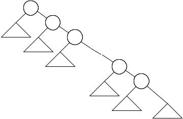
Figure 1.11. The only way this parse tree can evaluate to F. We represent parse trees for φ1, φ2, . . . , φn as triangles as their internal structure does not concern us here.
Step 1:
Definition 1.36 A formula of propositional logic φ is called a tautology i it evaluates to T under all its valuations, i.e. i φ.
Supposing that φ1, φ2, . . . , φn ψ holds, let us verify that φ1 → (φ2 → (φ3 → (. . . (φn → ψ) . . . ))) is indeed a tautology. Since the latter formula is a nested implication, it can evaluate to F only if all φ1, φ2,. . .,φn evaluate to T and ψ evaluates to F; see its parse tree in Figure 1.11. But this contradicts the fact that φ1, φ2, . . . , φn ψ holds. Thus, φ1 → (φ2 → (φ3 → (. . . (φn → ψ) . . . ))) holds.
Step 2:
Theorem 1.37 If η holds, then η is valid. In other words, if η is a tautology, then η is a theorem.
This step is the hard one. Assume that η holds. Given that η contains n distinct propositional atoms p1, p2, . . . , pn we know that η evaluates to T for all 2n lines in its truth table. (Each line lists a valuation of η.) How can we use this information to construct a proof for η? In some cases this can be done quite easily by taking a very good look at the concrete structure of η. But here we somehow have to come up with a uniform way of building such a proof. The key insight is to ‘encode’ each line in the truth table of η
1.4 Semantics of propositional logic |
51 |
as a sequent. Then we construct proofs for these 2n sequents and assemble them into a proof of η.
Proposition 1.38 Let φ be a formula such that p1, p2, . . . , pn are its only propositional atoms. Let l be any line number in φ’s truth table. For all 1 ≤ i ≤ n let pˆi be pi if the entry in line l of pi is T, otherwise pˆi is ¬pi. Then we have
1.pˆ1, pˆ2, . . . , pˆn φ is provable if the entry for φ in line l is T
2.pˆ1, pˆ2, . . . , pˆn ¬φ is provable if the entry for φ in line l is F
Proof: This proof is done by structural induction on the formula φ, that is, mathematical induction on the height of the parse tree of φ.
1.If φ is a propositional atom p, we need to show that p p and ¬p ¬p. These have one-line proofs.
2.If φ is of the form ¬φ1 we again have two cases to consider. First, assume that φ evaluates to T. In this case φ1 evaluates to F. Note that φ1 has the same atomic propositions as φ. We may use the induction hypothesis on φ1 to conclude that pˆ1, pˆ2, . . . , pˆn ¬φ1; but ¬φ1 is just φ, so we are done.
Second, if φ evaluates to F, then φ1 evaluates to T and we get pˆ1, pˆ2, . . . , pˆn φ1 by induction. Using the rule ¬¬i, we may extend the proof of pˆ1, pˆ2, . . . , pˆn φ1 to one for pˆ1, pˆ2, . . . , pˆn ¬¬φ1; but ¬¬φ1 is just ¬φ, so again we are done.
The remaining cases all deal with two subformulas: φ equals φ1 ◦ φ2, where ◦ is →, or . In all these cases let q1, . . . , ql be the propositional atoms of φ1 and r1, . . . , rk be the propositional atoms of φ2. Then we cer-
tainly have {q1, . . . , ql} {r1, . . . , rk } = {p1, . . . , pn}. Therefore, whenever qˆ1, . . . , qˆl ψ1 and rˆ1, . . . , rˆk ψ2 are valid so is pˆ1, . . . , pˆn ψ1 ψ2 using the rule i. In this way, we can use our induction hypothesis and only owe proofs that the conjunctions we conclude allow us to prove the desired conclusion for φ or ¬φ as the case may be.
3. To wit, let φ be φ1 → φ2. If φ evaluates to F, then we know that φ1 evaluates
to T and φ2 to F. Using our induction hypothesis, we |
have |
qˆ1, . . . , qˆl φ1 |
|
and rˆ1, . . . , rˆk ¬φ2, so |
pˆ1, . . . , pˆn φ1 ¬φ2 follows. |
We |
need to show |
pˆ1, . . . , pˆn ¬(φ1 → φ2); |
but using pˆ1, . . . , pˆn φ1 ¬φ2, this amounts to |
||
proving the sequent φ1 ¬φ2 ¬(φ1 → φ2), which we leave as an exercise.
If φ evaluates to T, then we have three cases. First, if φ1 evaluates to F and φ2 to F, then we get, by our induction hypothesis, that qˆ1, . . . , qˆl ¬φ1 and rˆ1, . . . , rˆk ¬φ2, so pˆ1, . . . , pˆn ¬φ1 ¬φ2 follows. Again, we need only to show the sequent ¬φ1 ¬φ2 φ1 → φ2, which we leave as an exercise. Second, if φ1 evaluates to F and φ2 to T, we use our induction hypothesis to arrive at
52 1 Propositional logic
pˆ1, . . . , pˆn ¬φ1 φ2 and have to prove ¬φ1 φ2 φ1 → φ2, which we leave as an exercise. Third, if φ1 and φ2 evaluate to T, we arrive at pˆ1, . . . , pˆn φ1 φ2, using our induction hypothesis, and need to prove φ1 φ2 φ1 → φ2, which we leave as an exercise as well.
4.If φ is of the form φ1 φ2, we are again dealing with four cases in total. First, if φ1 and φ2 evaluate to T, we get qˆ1, . . . , qˆl φ1 and rˆ1, . . . , rˆk φ2 by our induction hypothesis, so pˆ1, . . . , pˆn φ1 φ2 follows. Second, if φ1 evaluates to F and φ2 to T, then we get pˆ1, . . . , pˆn ¬φ1 φ2 using our induction hypothesis and the rule i as above and we need to prove ¬φ1 φ2 ¬(φ1 φ2), which we leave as an exercise. Third, if φ1 and φ2 evaluate to F, then our induction hypothesis and the rule i let us infer that pˆ1, . . . , pˆn ¬φ1 ¬φ2; so we are left with proving ¬φ1 ¬φ2 ¬(φ1 φ2), which we leave as an exercise. Fourth, if φ1 evaluates to T and φ2 to F, we obtain pˆ1, . . . , pˆn φ1 ¬φ2 by our induction hypothesis and we have to show φ1 ¬φ2 ¬(φ1 φ2), which we leave as an exercise.
5.Finally, if φ is a disjunction φ1 φ2, we again have four cases. First, if φ1 and φ2 evaluate to F, then our induction hypothesis and the rule i give us pˆ1, . . . , pˆn ¬φ1 ¬φ2 and we have to show ¬φ1 ¬φ2 ¬(φ1 φ2), which we leave as an exercise. Second, if φ1 and φ2 evaluate to T, then we obtain pˆ1, . . . , pˆn φ1 φ2, by our induction hypothesis, and we need a proof for φ1 φ2 φ1 φ2, which we leave as an exercise. Third, if φ1 evaluates to F and φ2 to T, then we arrive at pˆ1, . . . , pˆn ¬φ1 φ2, using our induction hypothesis, and need to establish ¬φ1 φ2 φ1 φ2, which we leave as an exercise. Fourth, if φ1 evaluates to T
and φ2 to F, then pˆ1, . . . , pˆn φ1 ¬φ2 results from our induction hypothesis and all we need is a proof for φ1 ¬φ2 φ1 φ2, which we leave as an
exercise. |
|
|
We apply this technique to the formula φ1 → (φ2 → (φ3 → (. . . (φn → ψ) . . . ))). Since it is a tautology it evaluates to T in all 2n lines of its truth table; thus, the proposition above gives us 2n many proofs of pˆ1, pˆ2, . . . , pˆn η, one for each of the cases that pˆi is pi or ¬pi. Our job now is to assemble all these proofs into a single proof for η which does not use any premises. We illustrate how to do this for an example, the tautology p q → p.
The formula p q → p has two propositional atoms p and q. By the proposition above, we are guaranteed to have a proof for each of the four sequents
p, q p q → p
¬p, q p q → p
p, ¬q p q → p
¬p, ¬q p q → p.
Ultimately, we want to prove p q → p by appealing to the four proofs of the sequents above. Thus, we somehow need to get rid of the premises on