→T

Figure 1.7. The evaluation of a logical formula under a given valuation.

Figure 1.8. An example of a truth table for a more complex logical formula.

Finally, column 7 results from applying the truth table of → to columns 5 and 6.

1.4.2 Mathematical induction

Here is a little anecdote about the German mathematician Gauss who, as a pupil at age 8, did not pay attention in class (can you imagine?), with the result that his teacher made him sum up all natural numbers from 1 to 100. The story has it that Gauss came up with the correct answer 5050 within seconds, which infuriated his teacher. How did Gauss do it? Well, possibly he knew that

for all natural numbers n.9 Thus, taking n = 100, Gauss could easily calculate:

1 + 2 + 3 + 4 + · · · + 100 = 100 · 101 = 5050. 2

Mathematical induction allows us to prove equations, such as the one in (1.5), for arbitrary n. More generally, it allows us to show that every natural number satisfies a certain property. Suppose we have a property M which we think is true of all natural numbers. We write M (5) to say that the property is true of 5, etc. Suppose that we know the following two things about the property M :

1.Base case: The natural number 1 has property M , i.e. we have a proof of M (1).

2.Inductive step: If n is a natural number which we assume to have property M (n), then we can show that n + 1 has property M (n + 1); i.e. we have a proof of M (n) → M (n + 1).

Definition 1.30 The principle of mathematical induction says that, on the grounds of these two pieces of information above, every natural number n has property M (n). The assumption of M (n) in the inductive step is called the induction hypothesis.

Why does this principle make sense? Well, take any natural number k. If k equals 1, then k has property M (1) using the base case and so we are done. Otherwise, we can use the inductive step, applied to n = 1, to infer that 2 = 1 + 1 has property M (2). We can do that using →e, for we know that 1 has the property in question. Now we use that same inductive step on n = 2 to infer that 3 has property M (3) and we repeat this until we reach n = k (see Figure 1.9). Therefore, we should have no objections about using the principle of mathematical induction for natural numbers.

Returning to Gauss’ example we claim that the sum 1 + 2 + 3 + 4 + · · · + n equals n · (n + 1)/2 for all natural numbers n.

Theorem 1.31 The sum 1 + 2 + 3 + 4 + · · · + n equals n · (n + 1)/2 for all natural numbers n.

9 There is another way of finding the sum 1 + 2 + · · · + 100, which works like this: write the sum backwards, as 100 + 99 + · · · + 1. Now add the forwards and backwards versions, obtaining 101 + 101 + · · · + 101 (100 times), which is 10100. Since we added the sum to itself, we now divide by two to get the answer 5050. Gauss probably used this method; but the method of mathematical induction that we explore in this section is much more powerful and can be applied in a wide variety of situations.

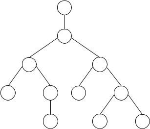
Figure 1.9. How the principle of mathematical induction works. By proving just two facts, M (1) and M (n) → M (n + 1) for a formal (and unconstrained) parameter n, we are able to deduce M (k) for each natural number k.

Proof: We use mathematical induction. In order to reveal the fine structure of our proof we write LHSn for the expression 1 + 2 + 3 + 4 + · · · + n and RHSn for n · (n + 1)/2. Thus, we need to show LHSn = RHSn for all n ≥ 1.

Base case: If n equals 1, then LHS1 is just 1 (there is only one summand), which happens to equal RHS1 = 1 · (1 + 1)/2.

Inductive step: Let us assume that LHSn = RHSn. Recall that this assumption is called the induction hypothesis; it is the driving force of our argument. We need to show LHSn+1 = RHSn+1, i.e. that the longer sum 1 + 2 + 3 + 4 + · · · + (n + 1) equals (n + 1) · ((n + 1) + 1)/2. The key observation is that the sum 1 + 2 + 3 + 4 + · · · + (n + 1) is nothing but the sum (1 + 2 + 3 + 4 + · · · + n) + (n + 1) of two summands, where the first one is the sum of our induction hypothesis. The latter says that 1 + 2 + 3 + 4 + · · · + n equals n · (n + 1)/2, and we are certainly entitled to substitute equals for equals in our reasoning. Thus, we compute

LHSn+1

=1 + 2 + 3 + 4 + · · · + (n + 1)

=LHSn + (n + 1) regrouping the sum

= RHSn + (n + 1) by our induction hypothesis

= RHSn+1.

Since we successfully showed the base case and the inductive step, we can use mathematical induction to infer that all natural numbers n have the property stated in the theorem above.

Actually, there are numerous variations of this principle. For example, we can think of a version in which the base case is n = 0, which would then cover all natural numbers including 0. Some statements hold only for all natural numbers, say, greater than 3. So you would have to deal with a base case 4, but keep the version of the inductive step (see the exercises for such an example). The use of mathematical induction typically suceeds on properties M (n) that involve inductive definitions (e.g. the definition of kl with l ≥ 0). Sentence (3) on page 2 suggests there may be true properties M (n) for which mathematical induction won’t work.

Course-of-values induction. There is a variant of mathematical induction in which the induction hypothesis for proving M (n + 1) is not just M (n), but the conjunction M (1) M (2) · · · M (n). In that variant, called course- of-values induction, there doesn’t have to be an explicit base case at all – everything can be done in the inductive step.

How can this work without a base case? The answer is that the base case is implicitly included in the inductive step. Consider the case n = 3: the inductive-step instance is M (1) M (2) M (3) → M (4). Now consider n = 1: the inductive-step instance is M (1) → M (2). What about the case when n equals 0? In this case, there are zero formulas on the left of the →, so we have to prove M (1) from nothing at all. The inductive-step instance is simply the obligation to show M (1). You might find it useful to modify Figure 1.9 for course-of-values induction.

Having said that the base case is implicit in course-of-values induction, it frequently turns out that it still demands special attention when you get inside trying to prove the inductive case. We will see precisely this in the two applications of course-of-values induction in the following pages.

¬

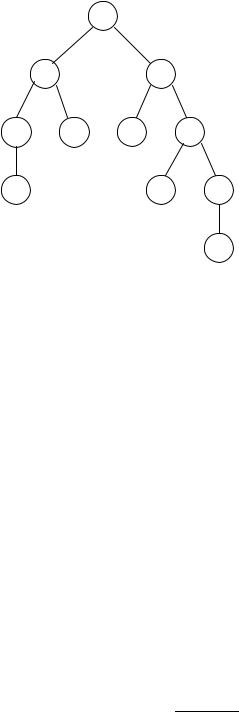
Figure 1.10. A parse tree with height 5.

In computer science, we often deal with finite structures of some kind, data structures, programs, files etc. Often we need to show that every instance of such a structure has a certain property. For example, the well-formed formulas of Definition 1.27 have the property that the number of ‘(’ brackets in a particular formula equals its number of ‘)’ brackets. We can use mathematical induction on the domain of natural numbers to prove this. In order to succeed, we somehow need to connect well-formed formulas to natural numbers.

Definition 1.32 Given a well-formed formula φ, we define its height to be 1 plus the length of the longest path of its parse tree.

For example, consider the well-formed formulas in Figures 1.3, 1.4 and 1.10. Their heights are 5, 6 and 5, respectively. In Figure 1.3, the longest path goes from → to to to ¬ to r, a path of length 4, so the height is 4 + 1 = 5. Note that the height of atoms is 1 + 0 = 1. Since every well-formed formula has finite height, we can show statements about all well-formed formulas by mathematical induction on their height. This trick is most often called structural induction, an important reasoning technique in computer science. Using the notion of the height of a parse tree, we realise that structural induction is just a special case of course-of-values induction.