x

Figure 6.7. A BDD where some boolean variables occur more than once on an evaluation path.

a variable the values 0 and 1 simultaneously.) Checking validity is similar, but we check that no 0-terminal is reachable by a consistent path.

The operations · and + can be performed by ‘surgery’ on the component BDDs. Given BDDs Bf and Bg representing boolean functions f and g, a BDD representing f · g can be obtained by taking the BDD f and replacing all its 1-terminals by Bg . To see why this is so, consider how to get to a 1-terminal in the resulting BDD. You have to satisfy the requirements for getting to a 1 imposed by both of the BDDs. Similarly, a BDD for f + g can be obtained by replacing all 0 terminals of Bf by Bg . Note that these operations are likely to generate BDDs with multiple occurrences of variables along a path. Later, in Section 6.2, we will see definitions of + and · on BDDs that don’t have this undesirable e ect.

The complementation operation ¯ is also possible: a BDD representing f can be obtained by replacing all 0-terminals in Bf by 1-terminals and vice versa. Figure 6.8 shows the complement of the BDD in Figure 6.2.

6.1.3 Ordered BDDs

We have seen that the representation of boolean functions by BDDs is often compact, thanks to the sharing of information a orded by the reductions C1–C3. However, BDDs with multiple occurrences of a boolean variable along a path seem rather ine cient. Moreover, there seems no easy way to test for equivalence of BDDs. For example, the BDDs of Figures 6.7 and 6.9 represent the same boolean function (the reader should check this). Neither of them can be optimised further by applying the rules C1–C3. However,

Figure 6.8. The complement of the BDD in Figure 6.2.

y y

0 1

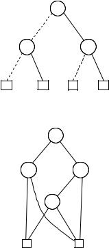
Figure 6.9. A BDD representing the same function as the BDD of Figure 6.7, but having the variable ordering [x, y, z].

testing whether they denote the same boolean function seems to involve as much computational e ort as computing the entire truth table for f (x, y, z).

We can improve matters by imposing an ordering on the variables occurring along any path. We then adhere to that same ordering for all the BDDs we manipulate.

Definition 6.6 Let [x1, . . . , xn] be an ordered list of variables without duplications and let B be a BDD all of whose variables occur somewhere in the list. We say that B has the ordering [x1, . . . , xn] if all variable labels of B occur in that list and, for every occurrence of xi followed by xj along any path in B, we have i < j.

An ordered BDD (OBDD) is a BDD which has an ordering for some list of variables.

Note that the BDDs of Figures 6.3(a,b) and 6.9 are ordered (with ordering [x, y]). We don’t insist that every variable in the list is used in the paths. Thus, the OBDDs of Figures 6.3 and 6.9 have the ordering [x, y, z] and so

0 1

Figure 6.10. A BDD which does not have an ordering of variables.

does any list having x, y and z in it in that order, such as [u, x, y, v, z, w] and [x, u, y, z]. Even the BDDs B0 and B1 in Figure 6.6 are OBDDs, a suitable ordering list being the empty list (there are no variables), or indeed any list. The BDD Bx of Figure 6.6(b) is also an OBDD, with any list containing x as its ordering.

The BDD of Figure 6.7 is not ordered. To see why this is so, consider the path taken if the values of x and y are 0. We begin with the root, an x- node, and reach a y-node and then an x-node again. Thus, no matter what list arrangement we choose (remembering that no double occurrences are allowed), this path violates the ordering condition. Another example of a BDD that is not ordered can be seen in Figure 6.10. In that case, we cannot find an order since the path for (x, y, z) (0, 0, 0) – meaning that x, y and z are assigned 0 – shows that y needs to occur before x in such a list, whereas the path for (x, y, z) (1, 1, 1) demands that x be before y.

It follows from the definition of OBDDs that one cannot have multiple occurrences of any variable along a path.

When operations are performed on two OBDDs, we usually require that they have compatible variable orderings. The orderings of B1 and B2 are said to be compatible if there are no variables x and y such that x comes before y in the ordering of B1 and y comes before x in the ordering of B2. This commitment to an ordering gives us a unique representation of boolean functions as OBDDs. For example, the BDDs in Figures 6.8 and 6.9 have compatible variable orderings.

Theorem 6.7 The reduced OBDD representing a given function f is unique. That is to say, let B and B be two reduced OBDDs with

x2 x2

1 0

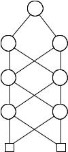
Figure 6.11. An OBDD for the even parity function for four bits.

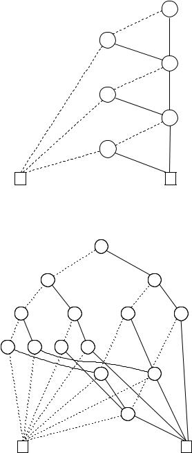
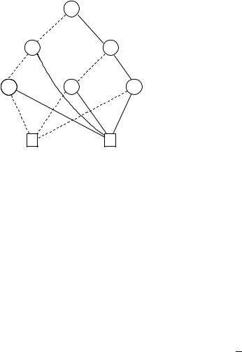
‘natural’ ordering [x1, x2, x3, x4, . . . ], then we can represent this function as an OBDD with 2n + 2 nodes. Figure 6.12 shows the resulting OBDD for n = 3. Unfortunately, if we choose instead the ordering

[x1, x3, . . . , x2n−1, x2, x4, . . . , x2n]

the resulting OBDD requires 2n+1 nodes; the OBDD for n = 3 can be seen in Figure 6.13.

The sensitivity of the size of an OBDD to the particular variable ordering is a price we pay for all the advantages that OBDDs have over BDDs. Although finding the optimal ordering is itself a computationally expensive problem, there are good heuristics which will usually produce a fairly good ordering. Later on we return to this issue in discussions of applications.

The importance of canonical representation The importance of having a canonical form for OBDDs in conjunction with an e cient test for deciding whether two reduced OBDDs are isomorphic cannot be overestimated. It allows us to perform the following tests:

Absence of redundant variables. If the value of the boolean function f (x1, x2, . . . , xn) does not depend on the value of xi, then any reduced OBDD which represents f does not contain any xi-node.

Test for semantic equivalence. If two functions f (x1, x2, . . . , xn) and g(x1, x2, . . . , xn) are represented by OBDDs Bf , respectively Bg , with a compatible ordering of variables, then we can e ciently decide whether f and g are semantically equivalent. We reduce Bf and Bg (if necessary); f