and g denote the same boolean functions if, and only if, the reduced OBDDs have identical structure.

Test for validity. We can test a function f (x1, x2, . . . , xn) for validity (i.e.

falways computes 1) in the following way. Compute a reduced OBDD for

f. Then f is valid if, and only if, its reduced OBDD is B1.

Test for implication. We can test whether f (x1, x2, . . . , xn) implies g(x1, x2, . . . , xn) (i.e. whenever f computes 1, then so does g) by computing the reduced OBDD for f · g. This is B0 i the implication holds.

Test for satisfiability. We can test a function f (x1, x2, . . . , xn) for satisfiability (f computes 1 for at least one assignment of 0 and 1 values to its variables). The function f is satisfiable i its reduced OBDD is not B0.

6.2 Algorithms for reduced OBDDs

6.2.1 The algorithm reduce

The reductions C1–C3 are at the core of any serious use of OBDDs, for whenever we construct a BDD we will want to convert it to its reduced form. In this section, we describe an algorithm reduce which does this e ciently for ordered BDDs.

If the ordering of B is [x1, x2, . . . , xl], then B has at most l + 1 layers. The algorithm reduce now traverses B layer by layer in a bottom-up fashion, beginning with the terminal nodes. In traversing B, it assigns an integer label id(n) to each node n of B, in such a way that the subOBDDs with root nodes n and m denote the same boolean function if, and only if, id(n) equals id(m).

Since reduce starts with the layer of terminal nodes, it assigns the first label (say #0) to the first 0-node it encounters. All other terminal 0-nodes denote the same function as the first 0-node and therefore get the same label (compare with reduction C1). Similarly, the 1-nodes all get the next label, say #1.

Now let us inductively assume that reduce has already assigned integer labels to all nodes of a layer > i (i.e. all terminal nodes and xj -nodes with j > i). We describe how nodes of layer i (i.e. xi-nodes) are being handled.

Definition 6.8 Given a non-terminal node n in a BDD, we define lo(n) to be the node pointed to via the dashed line from n. Dually, hi(n) is the node pointed to via the solid line from n.

Let us describe how the labelling is done. Given an xi-node n, there are three ways in which it may get its label:

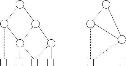
Figure 6.14. An example execution of the algorithm reduce.

If the label id(lo(n)) is the same as id(hi(n)), then we set id(n) to be that label. That is because the boolean function represented at n is the same function as the one represented at lo(n) and hi(n). In other words, node n performs a redundant test and can be eliminated by reduction C2.

If there is another node m such that n and m have the same variable xi, and id(lo(n)) = id(lo(m)) and id(hi(n)) = id(hi(m)), then we set id(n) to be id(m). This is because the nodes n and m compute the same boolean function (compare with reduction C3).

Otherwise, we set id(n) to the next unused integer label.

Note that only the last case creates a new label. Consider the OBDD in left side of Figure 6.14; each node has an integer label obtained in the manner just described. The algorithm reduce then finishes by redirecting edges bottom-up as outlined in C1–C3. The resulting reduced OBDD is in right of Figure 6.14. Since there are e cient bottom-up traversal algorithms for dags, reduce is an e cient operation in the number of nodes of an OBDD.

6.2.2 The algorithm apply

Another procedure at the heart of OBDDs is the algorithm apply. It is used to implement operations on boolean functions such as +, · , and complementation (via f 1). Given OBDDs Bf and Bg for boolean formulas f and g, the call apply (op, Bf , Bg ) computes the reduced OBDD of the boolean formula f op g, where op denotes any function from {0, 1} × {0, 1} to {0, 1}.

The intuition behind the apply algorithm is fairly simple. The algorithm operates recursively on the structure of the two OBDDs:

1.let v be the variable highest in the ordering (=leftmost in the list) which occurs in Bf or Bg .

2.split the problem into two subproblems for v being 0 and v being 1 and solve recursively;

3.at the leaves, apply the boolean operation op directly.

The result will usually have to be reduced to make it into an OBDD. Some reduction can be done ‘on the fly’ in step 2, by avoiding the creation of a new node if both branches are equal (in which case return the common result), or if an equivalent node already exists (in which case, use it).

Let us make all this more precise and detailed.

Definition 6.9 Let f be a boolean formula and x a variable.

1.We denote by f [0/x] the boolean formula obtained by replacing all occurrences of x in f by 0. The formula f [1/x] is defined similarly. The expressions f [0/x] and f [1/x] are called restrictions of f .

2.We say that two boolean formulas f and g are semantically equivalent if they represent the same boolean function (with respect to the boolean variables that they depend upon). In that case, we write f ≡ g.

def

For example, if f (x, y) = x · (y + x), then f [0/x](x, y) equals 0 · (y + 0), which is semantically equivalent to 0. Similarly, f [1/y](x, y) is x · (1 + x), which is semantically equivalent to x.

Restrictions allow us to perform recursion on boolean formulas, by decomposing boolean formulas into simpler ones. For example, if x is a variable in f , then f is equivalent to x · f [0/x] + x · f [1/x]. To see this, consider the case x = 0; the expression computes to f [0/x]. When x = 1 it yields f [1/x]. This observation is known as the Shannon expansion, although it can already be found in G. Boole’s book ‘The Laws of Thought’ from 1854.

Lemma 6.10 (Shannon expansion) For all boolean formulas f and all boolean variables x (even those not occurring in f ) we have

The function apply is based on the Shannon expansion for f op g:

This is used as a control structure of apply which proceeds from the roots

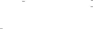
Figure 6.15. An example of two arguments for a call apply (+, Bf , Bg ).

of Bf and Bg downwards to construct nodes of the OBDD Bf op g . Let rf be the root node of Bf and rg the root node of Bg .

1. If both rf and rg are terminal nodes with labels lf and lg , respectively (recall that terminal labels are either 0 or 1), then we compute the value lf op lg and let the resulting OBDD be B0 if that value is 0 and B1 otherwise.

2.In the remaining cases, at least one of the root nodes is a non-terminal. Suppose that both root nodes are xi-nodes. Then we create an xi-node n with a dashed line to apply (op, lo(rf ), lo(rg )) and a solid line to apply (op, hi(rf ), hi(rg )), i.e.

we call apply recursively on the basis of (6.2).

3. If rf is an xi-node, but rg is a terminal node or an xj -node with j > i, then we know that there is no xi-node in Bg because the two OBDDs have a compatible ordering of boolean variables. Thus, g is independent of xi (g ≡ g[0/xi] ≡ g[1/xi]). Therefore, we create an xi-node n with a dashed line to apply (op, lo(rf ), rg ) and a solid line to apply (op, hi(rf ), rg ).

4.The case in which rg is a non-terminal, but rf is a terminal or an xj -node with j > i, is handled symmetrically to case 3.

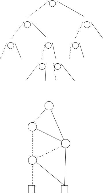
The result of this procedure might not be reduced; therefore apply finishes by calling the function reduce on the OBDD it constructed. An example of apply (where op is +) can be seen in Figures 6.15–6.17. Figure 6.16 shows the recursive descent control structure of apply and Figure 6.17 shows the final result. In this example, the result of apply (+, Bf , Bg ) is Bf .

Figure 6.16 shows that numerous calls to apply occur several times with the same arguments. E ciency could be gained if these were evaluated only

(R1, S1)

x1

Figure 6.16. The recursive call structure of apply for the example in Figure 6.15 (without memoisation).

x1

x2

x3

x4

Figure 6.17. The result of apply (+, Bf , Bg ), where Bf and Bg are given in Figure 6.15.