3.2 Linear-time temporal logic

Temporal logics have a dynamic aspect to them, since the truth of a formula is not fixed in a model, as it is in predicate or propositional logic, but depends on the time-point inside the model. In this chapter, we study a logic where time is linear, called Linear-time Temporal Logic (LTL), and another where time is branching, namely Computation Tree Logic (CTL). These logics have proven to be extremely fruitful in verifying hardware and communication protocols; and people are beginning to apply them to the verification of software. Model checking is the process of computing an answer to the question of whether M, s φ holds, where φ is a formula of one of these logics, M is an appropriate model of the system under consideration, s is a state of that model and is the underlying satisfaction relation.

Models like M should not be confused with an actual physical system. Models are abstractions that omit lots of real features of a physical system, which are irrelevant to the checking of φ. This is similar to the abstractions that one does in calculus or mechanics. There we talk about straight lines, perfect circles, or an experiment without friction. These abstractions are very powerful, for they allow us to focus on the essentials of our particular concern.

3.2 Linear-time temporal logic

Linear-time temporal logic, or LTL for short, is a temporal logic, with connectives that allow us to refer to the future. It models time as a sequence of states, extending infinitely into the future. This sequence of states is sometimes called a computation path, or simply a path. In general, the future is not determined, so we consider several paths, representing di erent possible futures, any one of which might be the ‘actual’ path that is realised.

We work with a fixed set Atoms of atomic formulas (such as p, q, r, . . . , or p1, p2, . . . ). These atoms stand for atomic facts which may hold of a system, like ÔPrinter Q5 is busy,Õ or ÔProcess 3259 is suspended,Õ or ÔThe content of register R1 is the integer value 6.Õ The choice of atomic descriptions obviously depends on our particular interest in a system at hand.

3.2.1 Syntax of LTL

Definition 3.1 Linear-time temporal logic (LTL) has the following syntax given in Backus Naur form:

φ ::= | | p | (¬φ) | (φ φ) | (φ φ) | (φ → φ)

where p is any propositional atom from some set Atoms.

FU

r

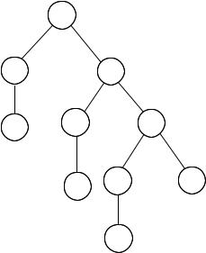
Figure 3.1. The parse tree of (F (p → G r) ((¬q) U p)).

Thus, the symbols and are LTL formulas, as are all atoms from Atoms; and ¬φ is an LTL formula if φ is one, etc. The connectives X, F, G, U, R, and W are called temporal connectives. X means ‘neXt state,’ F means ‘some Future state,’ and G means ‘all future states (Globally).’ The next three, U, R and W are called ‘Until,’ ‘Release’ and ‘Weak-until’ respectively. We will look at the precise meaning of all these connectives in the next section; for now, we concentrate on their syntax.

Here are some examples of LTL formulas:

(p W (q W r))

((G (F p)) → (F (q s))).

It’s boring to write all those brackets, and makes the formulas hard to read. Many of them can be omitted without introducing ambiguities; for example, (p → (F q)) could be written p → F q without ambiguity. Others, however, are required to resolve ambiguities. In order to omit some of those, we assume similar binding priorities for the LTL connectives to those we assumed for propositional and predicate logic.

→

q

Figure 3.2. The parse tree of F p → G r ¬q U p, assuming binding priorities of Convention 3.2.

Convention 3.2 The unary connectives (consisting of ¬ and the temporal connectives X, F and G) bind most tightly. Next in the order come U, R and W; then come and ; and after that comes →.

These binding priorities allow us to drop some brackets without introducing ambiguity. The examples above can be written:

F p G q → p W r

F (p → G r) ¬q U p

p W (q W r)

G F p → F (q s).

The brackets we retained were in order to override the priorities of Convention 3.2, or to disambiguate cases which the convention does not resolve. For example, with no brackets at all, the second formula would become F p → G r ¬q U p, corresponding to the parse tree of Figure 3.2, which is quite di erent.

The following are not well-formed formulas:

U r – since U is binary, not unary

p G q – since G is unary, not binary.

Definition 3.3 A subformula of an LTL formula φ is any formula ψ whose parse tree is a subtree of φ’s parse tree.

The subformulas of p W (q U r), e.g., are p, q, r, q U r and p W (q U r).

3.2.2 Semantics of LTL

The kinds of systems we are interested in verifying using LTL may be modelled as transition systems. A transition system models a system by means of states (static structure) and transitions (dynamic structure). More formally:

Definition 3.4 A transition system M = (S, →, L) is a set of states S endowed with a transition relation → (a binary relation on S), such that every s S has some s S with s → s , and a labelling function

L : S → P(Atoms).

Transition systems are also simply called models in this chapter. So a model has a collection of states S, a relation →, saying how the system can move from state to state, and, associated with each state s, one has the set of atomic propositions L(s) which are true at that particular state. We write P(Atoms) for the power set of Atoms, a collection of atomic descriptions. For example, the power set of {p, q} is { , {p}, {q}, {p, q}}. A good way of thinking about L is that it is just an assignment of truth values to all the propositional atoms, as it was the case for propositional logic (we called that a valuation). The di erence now is that we have more than one state, so this assignment depends on which state s the system is in: L(s) contains all atoms which are true in state s.

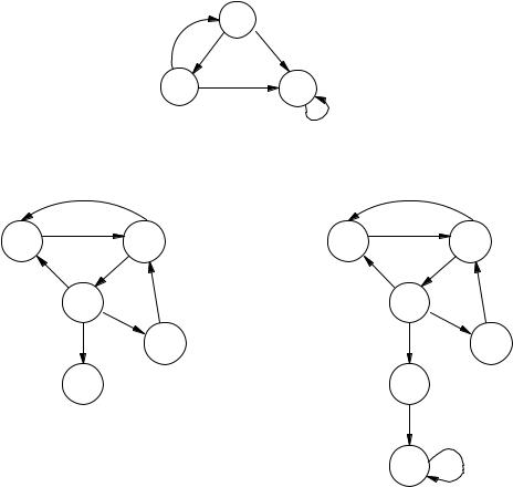
We may conveniently express all the information about a (finite) transition system M using directed graphs whose nodes (which we call states) contain all propositional atoms that are true in that state. For example, if our system has only three states s0, s1 and s2; if the only possible transi-

tions between states are s0 → s1, s0 → s2, s1 → s0, s1 → s2 and s2 → s2; and if L(s0) = {p, q}, L(s1) = {q, r} and L(s2) = {r}, then we can condense all this information into Figure 3.3. We prefer to present models by means of such pictures whenever that is feasible.

The requirement in Definition 3.4 that for every s S there is at least one s S such that s → s means that no state of the system can ‘deadlock.’ This is a technical convenience, and in fact it does not represent any real restriction on the systems we can model. If a system did deadlock, we could always add an extra state sd representing deadlock, together with new

sd

Figure 3.4. On the left, we have a system with a state s4 that does not have any further transitions. On the right, we expand that system with a ‘deadlock’ state sd such that no state can deadlock; of course, it is then our understanding that reaching the ‘deadlock’ state sd corresponds to deadlock in the original system.

transitions s → sd for each s which was a deadlock in the old system, as well as sd → sd. See Figure 3.4 for such an example.

Definition 3.5 A path in a model M = (S, →, L) is an infinite sequence of states s1, s2, s3, . . . in S such that, for each i ≥ 1, si → si+1. We write the path as s1 → s2 → . . . .

Consider the path π = s1 → s2 → . . . . It represents a possible future of our system: first it is in state s1, then it is in state s2, and so on. We write πi for the su x starting at si, e.g., π3 is s3 → s4 → . . . .

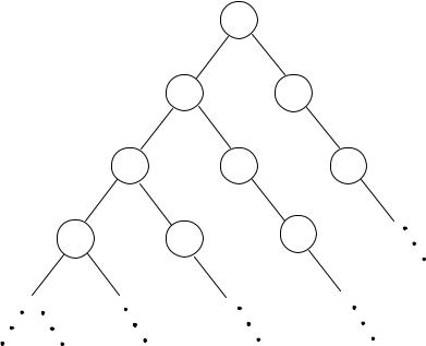
Figure 3.5. Unwinding the system of Figure 3.3 as an infinite tree of all computation paths beginning in a particular state.

It is useful to visualise all possible computation paths from a given state s by unwinding the transition system to obtain an infinite computation tree. For example, if we unwind the state graph of Figure 3.3 for the designated starting state s0, then we get the infinite tree in Figure 3.5. The execution paths of a model M are explicitly represented in the tree obtained by unwinding the model.

Definition 3.6 Let M = (S, →, L) be a model and π = s1 → . . . be a path in M. Whether π satisfies an LTL formula is defined by the satisfaction relation as follows:

1.π

2.π

3.π p i p L(s1)

4.π ¬φ i π φ

5.π φ1 φ2 i π φ1 and π φ2

6.π φ1 φ2 i π φ1 or π φ2

7.π φ1 → φ2 i π φ2 whenever π φ1

8.π X φ i π2 φ

9.π G φ i , for all i ≥ 1, πi φ

Figure 3.6. An illustration of the meaning of Until in the semantics of LTL. Suppose p is satisfied at (and only at) s3, s4, s5, s6, s7, s8 and q is satisfied at (and only at) s9. Only the states s3 to s9 each satisfy p U q along the path shown.

13.π φ R ψ i either there is some i ≥ 1 such that πi φ and for all j = 1, . . . , i we have πj ψ, or for all k ≥ 1 we have πk ψ.

Clauses 1 and 2 reflect the facts that is always true, and is always false. Clauses 3–7 are similar to the corresponding clauses we saw in propositional logic. Clause 8 removes the first state from the path, in order to create a path starting at the ‘next’ (second) state.

Notice that clause 3 means that atoms are evaluated in the first state along the path in consideration. However, that doesn’t mean that all the atoms occuring in an LTL formula refer to the first state of the path; if they are in the scope of a temporal connective, e.g., in G (p → X q), then the calculation of satisfaction involves taking su ces of the path in consideration, and the atoms refer to the first state of those su ces.

Let’s now look at clauses 11–13, which deal with the binary temporal connectives. U, which stands for ‘Until,’ is the most commonly encountered one of these. The formula φ1 U φ2 holds on a path if it is the case that φ1 holds continuously until φ2 holds. Moreover, φ1 U φ2 actually demands that φ2 does hold in some future state. See Figure 3.6 for illustration: each of the states s3 to s9 satisfies p U q along the path shown, but s0 to s2 don’t.

The other binary connectives are W, standing for ‘Weak-until,’ and R, standing for ‘Release.’ Weak-until is just like U, except that φ W ψ does not require that ψ is eventually satisfied along the path in question, which is required by φ U ψ. Release R is the dual of U; that is, φ R ψ is equivalent to ¬(¬φ U ¬ψ). It is called ‘Release’ because clause 11 determines that ψ must remain true up to and including the moment when φ becomes true (if there is one); φ ‘releases’ ψ. R and W are actually quite similar; the di erences are that they swap the roles of φ and ψ, and the clause for W has an i − 1

where R has i. Since they are similar, why do we need both? We don’t; they are interdefinable, as we will see later. However, it’s useful to have both. R is useful because it is the dual of U, while W is useful because it is a weak form of U.

Note that neither the strong version (U) or the weak version (W) of until says anything about what happens after the until has been realised. This is in contrast with some of the readings of ‘until’ in natural language. For example, in the sentence ‘I smoked until I was 22’ it is not only expressed that the person referred to continually smoked up until he or she was 22 years old, but we also would interpret such a sentence as saying that this person gave up smoking from that point onwards. This is di erent from the semantics of until in temporal logic. We could express the sentence about smoking by combining U with other connectives; for example, by asserting that it was once true that s U (t G ¬s), where s represents ‘I smoke’ and t represents ‘I am 22.’

Remark 3.7 Notice that, in clauses 9–13 above, the future includes the present. This means that, when we say ‘in all future states,’ we are including the present state as a future state. It is a matter of convention whether we do this, or not. As an exercise, you may consider developing a version of LTL in which the future excludes the present. A consequence of adopting the convention that the future shall include the present is that the formulas G p → p, p → q U p and p → F p are true in every state of every model.

So far we have defined a satisfaction relation between paths and LTL formulas. However, to verify systems, we would like to say that a model as a whole satisfies an LTL formula. This is defined to hold whenever every possible execution path of the model satisfies the formula.

Definition 3.8 Suppose M = (S, →, L) is a model, s S, and φ an LTL formula. We write M, s φ if, for every execution path π of M starting at s, we have π φ.

If M is clear from the context, we may abbreviate M, s φ by s φ. It should be clear that we have outlined the formal foundations of a procedure that, given φ, M and s, can check whether M, s φ holds. Later in this chapter, we will examine algorithms which implement this calculation. Let us now look at some example checks for the system in Figures 3.3 and 3.5.

1.M, s0 p q holds since the atomic symbols p and q are contained in the node of s0: π p q for every path π beginning in s0.