68 1 Propositional logic

in which φ is true. By our induction hypothesis, we know that all Pj and therefore P1 P2 · · · Pki have to be true in v as well. The conjunct P1 P2 · · · Pki → P of φ has be to true in v, too, from which we infer that P has to be true in v.

By mathematical induction, we therefore secured that (1.8) holds no matter how many cycles that while-statement went through.

Finally, we need to make sure that the if-statement above always renders correct replies. First, if is marked, then there has to be some conjunct P1 P2 · · · Pki → of φ such that all Pi are marked as well. By (1.8) that conjunct of φ evaluates to T → F = F whenever φ is true. As this is impossible the reply ‘unsatisfiable’ is correct. Second, if is not marked, we simply assign T to all marked atoms and F to all unmarked atoms and use proof by contradiction to show that φ has to be true with respect to that valuation.

If φ is not true under that valuation, it must make one of its principal conjuncts P1 P2 · · · Pki → P false. By the semantics of implication this can only mean that all Pj are true and P is false. By the definition of our valuation, we then infer that all Pj are marked, so P1 P2 · · · Pki → P is a conjunct of φ that would have been dealt with in one of the cycles of the while-statement and so P is marked, too. Since is not marked, P has to be or some atom q. In any event, the conjunct is then true by (1.8), a contradiction

Note that the proof by contradiction employed in the last proof was not really needed. It just made the argument seem more natural to us. The literature is full of such examples where one uses proof by contradiction more out of psychological than proof-theoretical necessity.

1.6 SAT solvers

The marking algorithm for Horn formulas computes marks as constraints on all valuations that can make a formule true. By (1.8), all marked atoms have to be true for any such valuation. We can extend this idea to general formulas φ by computing constraints saying which subformulas of φ require a certain truth value for all valuations that make φ true:

‘All marked subformulas evaluate to their mark value

In that way, marking atomic formulas generalizes to marking subformulas; and ‘true’ marks generalize into ‘true’ and ‘false’ marks. At the same

time, (1.9) serves as a guide for designing an algorithm and as an invariant for proving its correctness.

1.6.1 A linear solver

We will execute this marking algorithm on the parse tree of formulas, except that we will translate formulas into the adequate fragment

and then share common subformulas of the resulting parse tree, making the tree into a directed, acyclic graph (DAG). The inductively defined translation

transforms formulas generated by (1.3) into formulas generated by (1.10) such that φ and T (φ) are semantically equivalent and have the same propositional atoms. Therefore, φ is satisfiable i T (φ) is satisfiable; and the set of valuations for which φ is true equals the set of valuations for which T (φ) is true. The latter ensures that the diagnostics of a SAT solver, applied to T (φ), is meaningful for the original formula φ. In the exercises, you are asked to prove these claims.

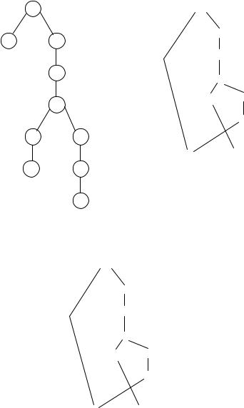
Example 1.48 For the formula φ being p ¬(q ¬p) we compute T (φ) = p ¬¬(¬q ¬¬p). The parse tree and DAG of T (φ) are depicted in Figure 1.12.

Any valuation that makes p ¬¬(¬q ¬¬p) true has to assign T to the topmost -node in its DAG of Figure 1.12. But that forces the mark T on the p-node and the topmost ¬-node. In the same manner, we arrive at a complete set of constraints in Figure 1.13, where the time stamps ‘1:’ etc indicate the order in which we applied our intuitive reasoning about these constraints; this order is generally not unique.

The formal set of rules for forcing new constraints from old ones is depicted in Figure 1.14. A small circle indicates any node (¬, or atom). The force laws for negation, ¬t and ¬f , indicate that a truth constraint on a ¬-node forces its dual value at its sub-node and vice versa. The law te propagates a T constraint on a -node to its two sub-nodes; dually, ti forces a T mark on a -node if both its children have that mark. The laws fl and fr force a F constraint on a -node if any of its sub-nodes has a F value. The laws fll

¬

¬¬

q¬

p

Figure 1.12. Parse tree (left) and directed acyclic graph (right) of the formula from Example 1.48. The p-node is shared on the right.

1: T

Figure 1.13. A witness to the satisfiability of the formula represented by this DAG.

and frr are more complex: if an -node has a F constraint and one of its sub-nodes has a T constraint, then the other sub-node obtains a F-constraint. Please check that all constraints depicted in Figure 1.13 are derivable from these rules. The fact that each node in a DAG obtained a forced marking does not yet show that this is a witness to the satisfiability of the formula

TT

Figure 1.14. Rules for flow of constraints in a formula’s DAG. Small circles indicate arbitrary nodes (¬, or atom). Note that the rules fll,frr and ti require that the source constraints of both = are present.

represented by this DAG. A post-processing phase takes the marks for all atoms and re-computes marks of all other nodes in a bottom-up manner, as done in Section 1.4 on parse trees. Only if the resulting marks match the ones we computed have we found a witness. Please verify that this is the case in Figure 1.13.

We can apply SAT solvers to checking whether sequents are valid. For example, the sequent p q → r p → q → r is valid i (p q → r) → p → q → r is a theorem (why?) i φ = ¬((p q → r) → p → q → r) is not satisfiable. The DAG of T (φ) is depicted in Figure 1.15. The annotations “1” etc indicate which nodes represent which sub-formulas. Notice that such DAGs may be constructed by applying the translation clauses for T to sub-formulas in a bottom-up manner – sharing equal subgraphs were applicable.

The findings of our SAT solver can be seen in Figure 1.16. The solver concludes that the indicated node requires the marks T and F for (1.9) to be met. Such contradictory constraints therefore imply that all formulas T (φ) whose DAG equals that of this figure are not satisfiable. In particular, all