

|
3.8 Exercises |
245 |
|
|
s1 |
|
s2 |
s0 |
|
|
|
q |
|
|
|
|
s3 |
p |
|
|
|
|
|
|
s4 |
q |
|
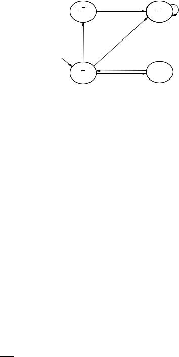
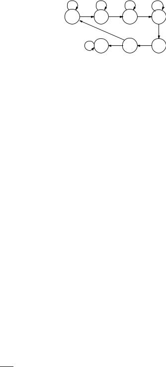
Figure 3.38. A system for which we compute invariants.
The other example we study is the computation of the set [[EG q]]. By Theorem 3.25, that set is the greatest fixed point of the function F above,
def
where φ = q. From Figure 3.38 we see that [[q]] = {s0, s4} and so F (X) = [[q]] ∩ pre (X) = {s0, s4} ∩ pre (X). Since [[EG q]] equals the greatest fixed
point of F , we need to iterate F on S until this process stabilises. First,
F 1(S) = {s0, s4} ∩ pre (S) = {s0, s4} ∩ S since every s has some s with s → s . Thus, F 1(S) = {s0, s4}.
Second, F 2(S) = F (F 1(S)) = {s0, s4} ∩ pre ({s0, s4}) = {s0, s4}. Therefore, {s0, s4} is the greatest fixed point of F , which equals [[EG q]] by Theo-
rem 3.25.
3.8 Exercises
Exercises 3.1
1.Read Section 2.7 in case you have not yet done so and classify Alloy and its constraint analyser according to the classification criteria for formal methods proposed on page 172.
2.Visit and browse the websites3 and4 to find formal methods that interest you for whatever reason. Then classify them according to the criteria from page 172.
Exercises 3.2
1.Draw parse trees for the LTL formulas:
(a)F p G q → p W r
(b)F (p → G r) ¬q U p
(c)p W (q W r)
(d)G F p → F (q s)
3www.afm.sbu.ac.uk
4www.cs.indiana.edu/formal-methods-education/
246 |
3 Verification by model checking |
|
|
q1 |
q2 |
|
ab |
ab |
ab |
ab |
q3 |
q4 |
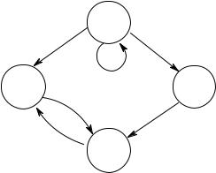
Figure 3.39. A model M.
2.Consider the system of Figure 3.39. For each of the formulas φ:
(a)G a
(b)a U b
(c)a U X (a ¬b)
(d)X ¬b G (¬a ¬b)
(e)X (a b) F (¬a ¬b)
(i)Find a path from the initial state q3 which satisfies φ.
(ii)Determine whether M, q3 φ.
3.Working from the clauses of Definition 3.1 (page 175), prove the equivalences:
φU ψ ≡ φ W ψ F ψ
φW ψ ≡ φ U ψ G φ
φW ψ ≡ ψ R (φ ψ)
φR ψ ≡ ψ W (φ ψ) .
4.Prove that φ U ψ ≡ ψ R (φ ψ) F ψ.
5. List all subformulas of the LTL formula ¬p U (F r G ¬q → q W ¬r).
6.‘Morally’ there ought to be a dual for W. Work out what it might mean, and then pick a symbol based on the first letter of the meaning.
7. Prove that for all paths π of all models, π φ W ψ F ψ implies π φ U ψ. That is, prove the remaining half of equivalence (3.2) on page 185.
8.Recall the algorithm NNF on page 62 which computes the negation normal form of propositional logic formulas. Extend this algorithm to LTL: you need to add program clauses for the additional connectives X, F, G and U, R and W; these clauses have to animate the semantic equivalences that we presented in this section.
3.8 Exercises |
247 |
Exercises 3.3
1.Consider the model in Figure 3.9 (page 193).
* (a) Verify that G(req -> F busy) holds in all initial states.
(b)Does ¬(req U ¬busy) hold in all initial states of that model?
(c)NuSMV has the capability of referring to the next value of a declared variable v by writing next(v). Consider the model obtained from Figure 3.9 by removing the self-loop on state !req & busy. Use the NuSMV feature next(...) to code that modified model as an NuSMV program with the specification G(req -> F busy). Then run it.
2.Verify Remark 3.11 from page 190.
* 3. Draw the transition system described by the ABP program.
Remarks: There are 28 reachable states of the ABP program. (Looking at the program, you can see that the state is described by nine boolean variables, namely
S.st, S.message1, S.message2, R.st, R.ack, R.expected, msg chan.output1, msg chan.output2 and finally ack chan.output. Therefore, there are 29 = 512 states in total. However, only 28 of them can be reached from the initial state by following a finite path.)
If you abstract away from the contents of the message (e.g., by setting S.message1 and msg chan.output1 to be constant 0), then there are only 12 reachable states. This is what you are asked to draw.
Exercises 3.4
1. Write the parse trees for the following CTL formulas:
*(a) EG r
*(b) AG (q → EG r)
*(c) A[p U EF r]
*(d) EF EG p → AF r, recall Convention 3.13
(e)A[p U A[q U r]]
(f)E[A[p U q] U r]
(g)AG (p → A[p U (¬p A[¬p U q])]).
2.Explain why the following are not well-formed CTL formulas:
*(a) F G r
(b)X X r
(c)A¬G ¬p
(d)F [r U q]
(e)EX X r
*(f) AEF r
*(g) AF [(r U q) (p U r)].
3.State which of the strings below are well-formed CTL formulas. For those which are well-formed, draw the parse tree. For those which are not well-formed, explain why not.
248 |
3 Verification by model checking |
s0 r
s1 |
p, t, r |
p, q |
s3 |
|
|
q, r
s2
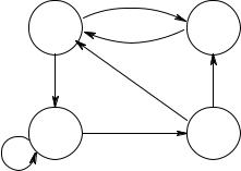
Figure 3.40. A model with four states.
(a)¬(¬p) (r s)
(b)X q
*(c) ¬AX q
(d)p U (AX )
*(e) E[(AX q) U (¬(¬p) ( s))]
*(f) (F r) (AG q)
(g)¬(AG q) (EG q).
* 4. List all subformulas of the formula AG (p → A[p U (¬p A[¬p U q])]).
5.Does E[req U ¬busy] hold in all initial states of the model in Figure 3.9 on page 193?
6.Consider the system M in Figure 3.40.
(a)Beginning from state s0, unwind this system into an infinite tree, and draw all computation paths up to length 4 (= the first four layers of that tree).
(b)Determine whether M, s0 φ and M, s2 φ hold and justify your answer, where φ is the LTL or CTL formula:
* (i) ¬p → r
(ii)F t
*(iii) ¬EG r
(iv)E (t U q)
(v)F q
(vi)EF q
(vii)EG r
(viii)G (r q).
7.Let M = (S, →, L) be any model for CTL and let [[φ]] denote the set of all s S such that M, s φ. Prove the following set identities by inspecting the clauses
of Definition 3.15 from page 211. * (a) [[ ]] = S,
(b)[[ ]] =
|
3.8 Exercises |
|
249 |
s0 |
p, q |
q, r |
s3 |
|
|
s1 |
|
s2 |
|
r |
p, t |
||
|
Figure 3.41. Another model with four states.
(c)[[¬φ]] = S − [[φ]],
(d)[[φ1 φ2]] = [[φ1]] ∩ [[φ2]]
(e)[[φ1 φ2]] = [[φ1]] [[φ2]]
* (f) [[φ1 → φ2]] = (S − [[φ1]]) [[φ2]] * (g) [[AX φ]] = S − [[EX ¬φ]]
(h)[[A(φ2 U φ2)]] = [[¬(E(¬φ1 U (¬φ1 ¬φ2)) EG ¬φ2)]].
8.Consider the model M in Figure 3.41. Check whether M, s0 φ and M, s2 φ hold for the CTL formulas φ:
(a)AF q
(b)AG (EF (p r))
(c)EX (EX r)
(d)AG (AF q).
* 9. The meaning of the temporal operators F, G and U in LTL and AU, EU, AG, EG, AF and EF in CTL was defined to be such that ‘the present includes the future.’ For example, EF p is true for a state if p is true for that state already. Often one would like corresponding operators such that the future excludes the present. Use suitable connectives of the grammar on page 208 to define such (six) modified connectives as derived operators in CTL.
10.Which of the following pairs of CTL formulas are equivalent? For those which are not, exhibit a model of one of the pair which is not a model of the other:
(a)EF φ and EG φ
*(b) EF φ EF ψ and EF (φ ψ)
*(c) AF φ AF ψ and AF (φ ψ)
(d)AF ¬φ and ¬EG φ
*(e) EF ¬φ and ¬AF φ
(f)A[φ1 U A[φ2 U φ3]] and A[A[φ1 U φ2] U φ3], hint: it might make it simpler if you think first about models that have just one path
(g)and AG φ → EG φ
*(h) and EG φ → AG φ.
11.Find operators to replace the ?, to make the following equivalences:

250 |
3 Verification by model checking |
*(a) AG (φ ψ) ≡ AG φ ? AG ψ
(b)EF ¬φ ≡ ¬??φ
12.State explicitly the meaning of the temporal connectives AR etc., as defined on page 217.
13.Prove the equivalences (3.6) on page 216.
* 14. Write pseudo-code for a recursive function TRANSLATE which takes as input an arbitrary CTL formula φ and returns as output an equivalent CTL formula ψ whose only operators are among the set { , ¬, , AF , EU , EX }.
Exercises 3.5
1.Express the following properties in CTL and LTL whenever possible. If neither is possible, try to express the property in CTL*:
* (a) Whenever p is followed by q (after finitely many steps), then the system enters an ‘interval’ in which no r occurs until t.
(b)Event p precedes s and t on all computation paths. (You may find it easier to code the negation of that specification first.)
(c)After p, q is never true. (Where this constraint is meant to apply on all computation paths.)
(d)Between the events q and r, event p is never true.
(e)Transitions to states satisfying p occur at most twice.
*(f) Property p is true for every second state along a path.
2.Explain in detail why the LTL and CTL formulas for the practical specification patterns of pages 183 and 215 capture the stated ‘informal’ properties expressed in plain English.
3.Consider the set of LTL/CTL formulas F = {F p → F q, AF p → AF q, AG (p → AF q)}.
(a)Is there a model such that all formulas hold in it?
(b)For each φ F, is there a model such that φ is the only formula in F satisfied in that model?
(c)Find a model in which no formula of F holds.
4.Consider the CTL formula AG (p → AF (s AX (AF t))). Explain what exactly it expresses in terms of the order of occurrence of events p, s and t.
5.Extend the algorithm NNF from page 62 which computes the negation normal form of propositional logic formulas to CTL*. Since CTL* is defined in terms of two syntactic categories (state formulas and path formulas), this requires two separate versions of NNF which call each other in a way that is reflected by the syntax of CTL* given on page 218.
6.Find a transition system which distinguishes the following pairs of CTL* formulas, i.e., show that they are not equivalent:
(a)AF G p and AF AG p
*(b) AG F p and AG EF p
(c)A[(p U r) (q U r)] and A[(p q) U r)]

3.8 Exercises |
251 |
*(d) A[X p X X p] and AX p AX AX p
(e)E[G F p] and EG EF p.
7.The translation from CTL with boolean combinations of path formulas to plain CTL introduced in Section 3.5.1 is not complete. Invent CTL equivalents for:
*(a) E[F p (q U r)]
*(b) E[F p G q].
In this way, we have dealt with all formulas of the form E[φ ψ]. Formulas of the form E[φ ψ] can be rewritten as E[φ] E[ψ] and A[φ] can be written ¬E[¬φ]. Use this translation to write the following in CTL:
(c)E[(p U q) F p]
*(d) A[(p U q) G p]
*(e) A[F p → F q].
8.The aim of this exercise is to demonstrate the expansion given for AW at the end of the last section, i.e., A[p W q] ≡ ¬E[¬q U ¬(p q)].
(a)Show that the following LTL formulas are valid (i.e., true in any state of any model):
(i)¬q U (¬p ¬q) → ¬G p
(ii)G ¬q F ¬p → ¬q U (¬p ¬q).
(b) Expand ¬((p U q) G p) using de Morgan rules and the LTL equivalence ¬(φ U ψ) ≡ (¬ψ U (¬φ ¬ψ)) ¬F ψ.
(c) Using your expansion and the facts (i) and (ii) above, show ¬((p U q) G p) ≡ ¬q U ¬(p q) and hence show that the desired expansion of AW above is correct.
Exercises 3.6
*1. Verify φ1 to φ4 for the transition system given in Figure 3.11 on page 198. Which of them require the fairness constraints of the SMV program in Figure 3.10?
2.Try to write a CTL formula that enforces non-blocking and no-strict-sequencing at the same time, for the SMV program in Figure 3.10 (page 196).
*3. Apply the labelling algorithm to check the formulas φ1, φ2, φ3 and φ4 of the mutual exclusion model in Figure 3.7 (page 188).
4.Apply the labelling algorithm to check the formulas φ1, φ2, φ3 and φ4 of the mutual exclusion model in Figure 3.8 (page 191).
5.Prove that (3.8) on page 228 holds in all models. Does your proof require that for every state s there is some state s with s → s ?
6.Inspecting the definition of the labelling algorithm, explain what happens if you perform it on the formula p ¬p (in any state, in any model).
7.Modify the pseudo-code for SAT on page 227 by writing a special procedure for
AG ψ1, without rewriting it in terms of other formulas5.
5Question: will your routine be more like the routine for AF, or more like that for EG on page 224? Why?

252 |
3 Verification by model checking |
*8. Write the pseudo-code for SATEG, based on the description in terms of deleting labels given in Section 3.6.1.
*9. For mutual exclusion, draw a transition system which forces the two processes
|
to enter their critical section in strict sequence and show that φ4 is false of its |
|
initial state. |
10. |
Use the definition of between states and CTL formulas to explain why s |
|
AG AF φ means that φ is true infinitely often along every path starting at s. |
* 11. |
Show that a CTL formula φ is true on infinitely many states of a computa- |
|
tion path s0 → s1 → s2 → . . . i for all n ≥ 0 there is some m ≥ n such that |
|
sm φ. |
12.Run the NuSMV system on some examples. Try commenting out, or deleting, some of the fairness constraints, if applicable, and see the counter examples NuSMV generates. NuSMV is very easy to run.
13.In the one-bit channel, there are two fairness constraints. We could have written this as a single one, inserting ‘&’ between running and the long formula, or we could have separated the long formula into two and made it into a total of three fairness constraints.
In general, what is the di erence between the single fairness constraint φ1 φ2
· · · φn and the n fairness constraints φ1, φ2, . . . , φn? Write an SMV program with a fairness constraint a & b which is not equivalent to the two fairness constraints a and b. (You can actually do it in four lines of SMV.)
14.Explain the construction of formula φ4, used to express that the processes need not enter their critical section in strict sequence. Does it rely on the fact that the safety property φ1 holds?
* 15. Compute the EC G labels for Figure 3.11, given the fairness constraints of the code in Figure 3.10 on page 196.
Exercises 3.7
1. Consider the functions
H1, H2, H3 : P({1, 2, 3, 4, 5, 6, 7, 8, 9, 10}) → P({1, 2, 3, 4, 5, 6, 7, 8, 9, 10})
defined by
def
H1(Y ) = Y − {1, 4, 7}
def
H2(Y ) = {2, 5, 9} − Y
def
H3(Y ) = {1, 2, 3, 4, 5} ∩ ({2, 4, 8} Y )
for all Y {1, 2, 3, 4, 5, 6, 7, 8, 9, 10}.
*(a) Which of these functions are monotone; which ones aren’t? Justify your answer in each case.
*(b) Compute the least and greatest fixed points of H3 using the iterations H3i with i = 1, 2, . . . and Theorem 3.24.
3.8 Exercises |
253 |
q
q |
q |
p |
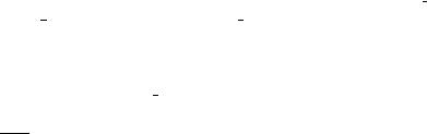
Figure 3.42. Another system for which we compute invariants.
(c)Does H2 have any fixed points?
(d)Recall G : P({s0, s1}) → P({s0, s1}) with
|
|
def |
{s0} then {s1} else {s0} . |
|
|||
|
|
G(Y ) = if Y = |
|
||||
|
|
Use mathematical induction to show that Gi equals G for all odd numbers |
|||||
|
|
i ≥ 1. What does Gi look like for even numbers i? |
|
|
|||
* |
2. |
Let A and B be two subsets of S and let F : P(S) → P(S) be a monotone |
|||||
|
|
function. Show that: |
|
|
|
|
|
|
|
def |
A |
|
F (Y ) is monotone; |
|
|
|
|
= |
∩ |
|
|
||
|
|
(a) F1 : P(S) → P(S) with F1(Y ) def |
|
|
|
|
|
|
|
(b) F2 : P(S) → P(S) with F2(Y ) = |
A (B ∩ F (Y )) is monotone. |
|
|||
|
3. |
Use Theorems 3.25 and 3.26 to compute the following sets (the underlying model |
|||||
|
|
is in Figure 3.42): |
|
|
|
|
|
|
|
(a) [[EF p]] |
|
|
|
|
|
|
|
(b) [[EG q]]. |
|
|
|
|
|
|
4. |
Using the function F (X) = [[φ]] pre (X) prove that [[AF φ]] is the least fixed |
|||||
|
|
point of F . Hence argue that the procedure SATAF is correct and terminates. |
|||||
* |
5. |
One may also compute AG φ directly as a fixed point. Consider the function |
|||||
|
|
H : P(S) → P(S) with H(X) = [[φ]] ∩ pre (X). Show that H is monotone and |
|||||
|
|
that [[AG φ]] is the greatest fixed point of H. Use that insight to write a procedure |
|||||
|
|
SATAG. |
|
|
|
|
|
|
6. |
Similarly, one may compute A[φ1 U φ2] directly as a |
fixed point, |
using |
|||
|
|
K : P(S) → P(S), where K(X) = [[φ2]] ([[φ1]] ∩ pre (X)). |
Show that |
K is |
|||
monotone and that [[A[φ1 U φ2]]] is the least fixed point of K. Use that insight to write a procedure SATAU. Can you use that routine to handle all calls of the form AF φ as well?
7.Prove that [[A[φ1 U φ2]]] = [[φ2 (φ1 AX (A[φ1 U φ2]))]].
8.Prove that [[AG φ]] = [[φ AX (AG φ)]].
9.Show that the repeat-statements in the code for SATEU and SATEG always terminate. Use this fact to reason informally that the main program SAT terminates for all valid CTL formulas φ. Note that some subclauses, like the one for AU, call SAT recursively and with a more complex formula. Why does this not a ect termination?