Binary decision diagrams

Example 6.2 In terms of the four functions above, we can define other boolean functions such as

def

(1) f (x, y) = x · (y + x)

def

(2) g(x, y) = x · y + (1 x)

def

(3) h(x, y, z) = x + y · (x y)

def

(4) k() = 1 (0 · 1).

6.1.1 Propositional formulas and truth tables

Truth tables and propositional formulas are two di erent representations of boolean functions. In propositional formulas, denotes ·, denotes +, ¬ denotes ¯ and and denote 1 and 0, respectively.

Boolean functions are represented by truth tables in the obvious way; for

On the right, we show the same truth table using the notation of Chapter 1; a formula having this truth table is ¬(p q). In this chapter, we may mix these two notational systems of boolean formulas and formulas of propositional logic whenever it is convenient. You should be able to translate expressions easily from one notation to the other and vice versa.

As representations of boolean functions, propositional formulas and truth tables have di erent advantages and disadvantages. Truth tables are very space-ine cient: if one wanted to model the functionality of a sequential circuit by a boolean function of 100 variables (a small chip component would easily require this many variables), then the truth table would require 2100 (which is more than 1030) lines. Alas, there is not enough storage space (whether paper or particle) in the universe to record the information of 2100 di erent bit vectors of length 100. Although they are space ine cient, operations on truth tables are simple. Once you have computed a truth table, it is easy to see whether the boolean function represented is satisfiable: you just look to see if there is a 1 in the last column of the table.

Comparing whether two truth tables represent the same boolean function also seems easy: assuming the two tables are presented with the same order

of valuations, we simply check that they are identical. Although these operations seem simple, however, they are computationally intractable because of the fact that the number of lines in the truth table is exponential in the number of variables. Checking satisfiability of a function with n atoms requires of the order of 2n operations if the function is represented as a truth table. We conclude that checking satisfiability and equivalence is highly ine cient with the truth-table representation.

Representation of boolean functions by propositional formulas is slightly better. Propositional formulas often provide a wonderfully compact and e - cient presentation of boolean functions. A formula with 100 variables might only be about 200–300 characters long. However, deciding whether an arbitrary propositional formula is satisfiable is a famous problem in computer science: no e cient algorithms for this task are known, and it is strongly suspected that there aren’t any. Similarly, deciding whether two arbitrary propositional formulas f and g denote the same boolean function is suspected to be exponentially expensive.

It is straightforward to see how to perform the boolean operations ·, +, and ¯ on these two representations. In the case of truth tables, they involve applying the operation to each line; for example, given truth tables for f and g over the same set of variables (and in the same order), the truth table for f g is obtained by applying to the truth value of f and g in each line. If f and g do not have the same set of arguments, it is easy to pad them out by adding further arguments. In the case of representation by propositional formulas, the operations ·, , etc., are simply syntactic manipulations. For example, given formulas φ and ψ representing the functions f and g, the formulas representing f · g and f g are, respectively, φ ψ and (φ ¬ψ) (¬φ ψ).

We could also consider representing boolean functions by various subclasses of propositional formulas, such as conjunctive and disjunctive normal forms. In the case of disjunctive normal form (DNF, in which a formula is a disjunction of conjunctions of literals), the representation is sometimes compact, but in the worst cases it can be very lengthy. Checking satisfiability is a straightforward operation, however, because it is su cient to find a disjunct which does not have two complementary literals. Unfortunately, there is not a similar way of checking validity. Performing + on two formulas in DNF simply involves inserting between them. Performing · is more complicated; we cannot simply insert between the two formulas, because the result will not in general be in DNF, so we have to perform lengthy applications of the distributivity rule φ (ψ1 ψ2) ≡ (φ ψ1) (φ ψ1). Computing the negation of a DNF formula is also expensive. The DNF formula φ may be

Figure 6.1. Comparing efficiency of five representations of boolean formulas.

y y

Figure 6.2. An example of a binary decision tree.

quite short, whereas the length of the disjunctive normal form of ¬φ can be exponential in the length of φ.

The situation for representation in conjunctive normal form is the dual. A summary of these remarks is contained in Figure 6.1 (for now, please ignore the last row).

6.1.2 Binary decision diagrams

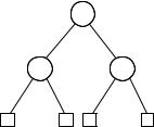
Binary decision diagrams (BDDs) are another way of representing boolean functions. A certain class of such diagrams will provide the implementational framework for our symbolic model-checking algorithm. Binary decision diagrams were first considered in a simpler form called binary decision trees. These are trees whose non-terminal nodes are labelled with boolean variables x, y, z, . . . and whose terminal nodes are labelled with either 0 or 1. Each non-terminal node has two edges, one dashed line and one solid line. In Figure 6.2 you can see such a binary decision tree with two layers of variables x and y.

Definition 6.3 Let T be a finite binary decision tree. Then T determines a unique boolean function of the variables in non-terminal nodes, in the following way. Given an assignment of 0s and 1s to the boolean variables

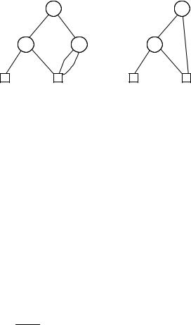
Figure 6.3. (a) Sharing the terminal nodes of the binary decision tree in Figure 6.2; (b) further optimisation by removing a redundant decision point.

occurring in T , we start at the root of T and take the dashed line whenever the value of the variable at the current node is 0; otherwise, we travel along the solid line. The function value is the value of the terminal node we reach.

For example, the binary decision tree of Figure 6.2 represents a boolean function f (x, y). To find f (0, 1), start at the root of the tree. Since the value of x is 0 we follow the dashed line out of the node labelled x and arrive at the leftmost node labelled y. Since y’s value is 1, we follow the solid line out of that y-node and arrive at the leftmost terminal node labelled 0. Thus, f (0, 1) equals 0. In computing f (0, 0), we similarly travel down the tree, but now following two dashed lines to obtain 1 as a result. You can see that the two other possibilities result in reaching the remaining two terminal nodes labelled 0. Thus, this binary decision tree computes the

def

function f (x, y) = x + y.

Binary decision trees are quite close to the representation of boolean functions as truth tables as far as their sizes are concerned. If the root of a binary decision tree is an x-node then it has two subtrees (one for the value of x being 0 and another one for x having value 1). So if f depends on n boolean variables, the corresponding binary decision tree will have at least 2n+1 − 1 nodes (see exercise 5 on page 399). Since f ’s truth table has 2n lines, we see that decision trees as such are not a more compact representation of boolean functions. However, binary decision trees often contain some redundancy which we can exploit.

Since 0 and 1 are the only terminal nodes of binary decision trees, we can optimise the representation by having pointers to just one copy of 0 and one copy of 1. For example, the binary decision tree in Figure 6.2 can be optimised in this way and the resulting structure is depicted in Figure 6.3(a). Note that we saved storage space for two redundant terminal 0-nodes, but that we still have as many edges (pointers) as before.

Figure 6.6. The BDDs (a) B0, representing the constant 0 boolean function; similarly, the BDD B1 has only one node 1 and represents the constant 1 boolean function; and (b) Bx, representing the boolean variable x.

non-terminal node has exactly two edges from that node to others: one labelled 0 and one labelled 1 (we represent them as a dashed line and a solid line, respectively).

A BDD is said to be reduced if none of the optimisations C1–C3 can be applied (i.e. no more reductions are possible).

All the decision structures we have seen in this chapter (Figures 6.2–6.5) are BDDs, as are the constant functions B0 and B1, and the function Bx from Figure 6.6. If B is a BDD where V = {x1, x2, . . . , xn} is the set of labels of non-terminal nodes, then B determines a boolean function f (V ) in the same way as binary decision trees (see Definition 6.3): given an assignment of 0s and 1s to the variables in V , we compute the value of f by starting with the unique initial node. If its variable has value 0, we follow the dashed line; otherwise we take the solid line. We continue for each node until we reach a terminal node. Since the BDD is finite by definition, we eventually reach a terminal node which is labelled with 0 or 1. That label is the result of f for that particular assignment of truth values.

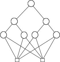
The definition of a BDD does not prohibit that a boolean variable occur more than once on a path in the dag. For example, consider the BDD in Figure 6.7.

Such a representation is wasteful, however. The solid link from the leftmost x to the 1-terminal is never taken, for example, because one can only get to that x-node when x has value 0.

Thanks to the reductions C1–C3, BDDs can often be quite compact representations of boolean functions. Let us consider how to check satisfiability and perform the boolean operations on functions represented as BDDs. A BDD represents a satisfiable function if a 1-terminal node is reachable from the root along a consistent path in a BDD which represents it. A consistent path is one which, for every variable, has only dashed lines or only solid lines leaving nodes labelled by that variable. (In other words, we cannot assign