3.4.3 Practical patterns of specifications

It’s useful to look at some typical examples of formulas, and compare the situation with LTL (Section 3.2.3). Suppose atomic descriptions include some words such as busy and requested.

It is possible to get to a state where started holds, but ready doesn’t:

EF (started ¬ready). To express impossibility, we simply negate the formula.

For any state, if a request (of some resource) occurs, then it will eventually be acknowledged:

AG (requested → AF acknowledged).

The property that if the process is enabled infinitely often, then it runs infinitely often, is not expressible in CTL. In particular, it is not expressed by AG AF enabled → AG AF running, or indeed any other insertion of A or E into the corresponding LTL formula. The CTL formula just given expresses that if every path has infinitely often enabled, then every path is infinitely often taken; this is much weaker than asserting that every path which has infinitely often enabled is infinitely often taken.

A certain process is enabled infinitely often on every computation path: AG (AF enabled).

Whatever happens, a certain process will eventually be permanently deadlocked: AF (AG deadlock).

From any state it is possible to get to a restart state: AG (EF restart).

An upwards travelling lift at the second floor does not change its direction when it has passengers wishing to go to the fifth floor:

AG (floor2 directionup ButtonPressed5 → A[directionup U floor5])

Here, our atomic descriptions are boolean expressions built from system variables, e.g., floor2.

The lift can remain idle on the third floor with its doors closed: AG (floor3 idle doorclosed → EG (floor3 idle doorclosed)).

A process can always request to enter its critical section. Recall that this was not expressible in LTL. Using the propositions of Figure 3.8, this may be written AG (n1 → EX t1) in CTL.

Processes need not enter their critical section in strict sequence. This was also not expressible in LTL, though we expressed its negation. CTL allows us to express it directly: EF (c1 E[c1 U (¬c1 E[¬c2 U c1])]).

3.4.4Important equivalences between CTL formulas

Definition 3.16 Two CTL formulas φ and ψ are said to be semantically equivalent if any state in any model which satisfies one of them also satisfies the other; we denote this by φ ≡ ψ.

We have already noticed that A is a universal quantifier on paths and E is the corresponding existential quantifier. Moreover, G and F are also universal and existential quantifiers, ranging over the states along a particular path. In view of these facts, it is not surprising to find that de Morgan rules exist:

¬AF φ ≡ EG ¬φ

¬AX φ ≡ EX ¬φ.

We also have the equivalences

AF φ ≡ A[ U φ] EF φ ≡ E[ U φ]

which are similar to the corresponding equivalences in LTL.

3.4.5 Adequate sets of CTL connectives

As in propositional logic and in LTL, there is some redundancy among the CTL connectives. For example, the connective AX can be written ¬EX ¬; and AG, AF, EG and EF can be written in terms of AU and EU as follows: first, write AG φ as ¬EF ¬φ and EG φ as ¬AF ¬φ, using (3.6), and then use AF φ ≡ A[ U φ] and EF φ ≡ E[ U φ]. Therefore AU, EU and EX form an adequate set of temporal connectives.

Also EG, EU, and EX form an adequate set, for we have the equivalence

which can be proved as follows:

A[φ U ψ] ≡ A[¬(¬ψ U (¬φ ¬ψ)) F ψ]

≡¬E¬[¬(¬ψ U (¬φ ¬ψ)) F ψ]

≡¬E[(¬ψ U (¬φ ¬ψ)) G ¬ψ]

≡¬(E[¬ψ U (¬φ ¬ψ)] EG ¬ψ).

The first line is by Theorem 3.10, and the remainder by elementary manipulation. (This proof involves intermediate formulas which violate the syntactic formation rules of CTL; however, it is valid in the logic CTL* introduced in the next section.) More generally, we have:

Theorem 3.17 A set of temporal connectives in CTL is adequate if, and only if, it contains at least one of {AX , EX }, at least one of {EG , AF , AU } and EU .

This theorem is proved in a paper referenced in the bibliographic notes at the end of the chapter. The connective EU plays a special role in that theorem because neither weak-until W nor release R are primitive in CTL (Definition 3.12). The temporal connectives AR, ER, AW and EW are all definable in CTL:

A[φ R ψ] = ¬E[¬φ U ¬ψ]

E[φ R ψ] = ¬A[¬φ U ¬ψ]

These definitions are justified by LTL equivalences in Sections 3.2.4 and 3.2.5. Some other noteworthy equivalences in CTL are the following:

AG φ ≡ φ AX AG φ

EG φ ≡ φ EX EG φ

AF φ ≡ φ AX AF φ

EF φ ≡ φ EX EF φ

A[φ U ψ] ≡ ψ (φ AX A[φ U ψ])

E[φ U ψ] ≡ ψ (φ EX E[φ U ψ]).

For example, the intuition for the third one is the following: in order to have AF φ in a particular state, φ must be true at some point along each path from that state. To achieve this, we either have φ true now, in the current state; or we postpone it, in which case we must have AF φ in each of the next states. Notice how this equivalence appears to define AF in terms of AX and AF itself, an apparently circular definition. In fact, these equivalences can be used to define the six connectives on the left in terms of AX and EX , in a non-circular way. This is called the fixed-point characterisation of CTL; it is the mathematical foundation for the model-checking algorithm developed in Section 3.6.1; and we return to it later (Section 3.7).

3.5 CTL* and the expressive powers of LTL and CTL

CTL allows explicit quantification over paths, and in this respect it is more expressive than LTL, as we have seen. However, it does not allow one to select a range of paths by describing them with a formula, as LTL does. In that respect, LTL is more expressive. For example, in LTL we can say ‘all paths which have a p along them also have a q along them,’ by writing F p → F q. It is not possible to write this in CTL because of the constraint that every F has an associated A or E. The formula AF p → AF q means

something quite di erent: it says ‘if all paths have a p along them, then all paths have a q along them.’ One might write AG (p → AF q), which is closer, since it says that every way of extending every path to a p eventually meets a q, but that is still not capturing the meaning of F p → F q.

CTL* is a logic which combines the expressive powers of LTL and CTL, by dropping the CTL constraint that every temporal operator (X, U, F, G) has to be associated with a unique path quantifier (A, E). It allows us to write formulas such as

These formulas are not equivalent to, respectively, A[(p q) U r)], AX p AX AX p and EG EF p. It turns out that the first of them can be written as a (rather long) CTL formula. The second and third do not have a CTL equivalent.

The syntax of CTL* involves two classes of formulas:

state formulas, which are evaluated in states:

φ::= | p | (¬φ) | (φ φ) | A[α] | E[α]

where p is any atomic formula and α any path formula; and

path formulas, which are evaluated along paths:

α::= φ | (¬α) | (α α) | (α U α) | (G α) | (F α) | (X α)

where φ is any state formula. This is an example of an inductive definition which is mutually recursive: the definition of each class depends upon the definition of the other, with base cases p and .

LTL and CTL as subsets of CTL* Although the syntax of LTL does not include A and E, the semantic viewpoint of LTL is that we consider all paths. Therefore, the LTL formula α is equivalent to the CTL* formula A[α]. Thus, LTL can be viewed as a subset of CTL*.

CTL is also a subset of CTL*, since it is the fragment of CTL* in which we restrict the form of path formulas to

α ::= (φ U φ) | (G φ) | (F φ) | (X φ)

Figure 3.23 shows the relationship among the expressive powers of CTL, LTL and CTL*. Here are some examples of formulas in each of the subsets

CTL*

LTL

Figure 3.23. The expressive powers of CTL, LTL and CTL*.

shown:

def

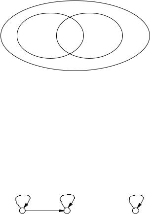
In CTL but not in LTL: ψ1 = AG EF p. This expresses: wherever we have got to, we can always get to a state in which p is true. This is also useful, e.g., in finding deadlocks in protocols.

The proof that AG EF p is not expressible in LTL is as follows. Let φ be an LTL formula such that A[φ] is allegedly equivalent to AG EF p. Since M, s AG EF p in the left-hand diagram below, we have M, s A[φ]. Now let M be as shown in the right-hand diagram. The paths from s in M are a subset of those from s in M, so we have M , s A[φ]. Yet, it is not the case that M , s AG EF p; a contradiction.

def

In CTL*, but neither in CTL nor in LTL: ψ4 = E[G F p], saying that there is a path with infinitely many p.

The proof that this is not expressible in CTL is quite complex and may be found in the papers co-authored by E. A. Emerson with others, given in the references. (Why is it not expressible in LTL?)

def

In LTL but not in CTL: ψ3 = A[G F p → F q], saying that if there are infinitely many p along the path, then there is an occurrence of q. This is an interesting thing to be able to say; for example, many fairness constraints are of the form ‘infinitely often requested implies eventually acknowledged’.

def

In LTL and CTL: ψ2 = AG (p → AF q) in CTL, or G (p → F q) in LTL: any p is eventually followed by a q.

Remark 3.18 We just saw that some (but not all) LTL formulas can be converted into CTL formulas by adding an A to each temporal operator. For