will analyse the code in the file counter3.smv and report on the specifications it contains. One can also run NuSMV interactively. In that case, the command line

NuSMV -int counter3.smv

enters NuSMV’s command-line interpreter. From there, there is a variety of commands you can use which allow you to compile the description and run the specification checks, as well as inspect partial results and set various parameters. See the NuSMV user manual for more details.

NuSMV also supports bounded model checking, invoked by the commandline option -bmc. Bounded model checking looks for counterexamples in order of size, starting with counterexamples of length 1, then 2, etc., up to a given threshold (10 by default). Note that bounded model checking is incomplete: failure to find a counterexample does not mean that there is none, but only that there is none of length up to the threshold. For related reasons, this incompleteness features also in Alloy and its constraint analyzer. Thus, while a negative answer can be relied on (if NuSMV finds a counterexample, it is valid), a positive one cannot. References on bounded model checking can be found in the bibliographic notes on page 254. Later on, we use bounded model checking to prove the optimality of a scheduler.

3.3.4 Mutual exclusion revisited

Figure 3.10 gives the SMV code for a mutual exclusion protocol. This code consists of two modules, main and prc. The module main has the variable turn, which determines whose turn it is to enter the critical section if both are trying to enter (recall the discussion about the states s3 and s9 in Section 3.3.1).

The module main also has two instantiations of prc. In each of these instantiations, st is the status of a process (saying whether it is in its critical section, or not, or trying) and other-st is the status of the other process (notice how this is passed as a parameter in the third and fourth lines of main).

The value of st evolves in the way described in a previous section: when it is n, it may stay as n or move to t. When it is t, if the other one is n, it will go straight to c, but if the other one is t, it will check whose turn it is before going to c. Then, when it is c, it may move back to n. Each instantiation of prc gives the turn to the other one when it gets to its critical section.

An important feature of SMV is that we can restrict its search tree to execution paths along which an arbitrary boolean formula about the state

-- ‘negation’ of strict sequencing (desired to be false) LTLSPEC G(pr1.st=c -> ( G pr1.st=c | (pr1.st=c U

Figure 3.10. SMV code for mutual exclusion. Because W is not supported by SMV, we had to make use of equivalence (3.3) to write the no-strict-sequencing formula as an equivalent but longer formula involving U.

φ is true infinitely often. Because this is often used to model fair access to resources, it is called a fairness constraint and introduced by the keyword FAIRNESS. Thus, the occurrence of FAIRNESS φ means that SMV, when checking a specification ψ, will ignore any path along which φ is not satisfied infinitely often.

In the module prc, we restrict model checks to computation paths along which st is infinitely often not equal to c. This is because our code allows the process to stay in its critical section as long as it likes. Thus, there is another opportunity for liveness to fail: if process 2 stays in its critical section forever, process 1 will never be able to enter. Again, we ought not to take this kind of violation into account, since it is patently unfair if a process is allowed to stay in its critical section for ever. We are looking for more subtle violations of the specifications, if there are any. To avoid the one above, we stipulate the fairness constraint !(st=c).

If the module in question has been declared with the process keyword, then at each time point SMV will non-deterministically decide whether or not to select it for execution, as explained earlier. We may wish to ignore paths in which a module is starved of processor time. The reserved word running can be used instead of a formula in a fairness constraint: writing FAIRNESS running restricts attention to execution paths along which the module in which it appears is selected for execution infinitely often.

In prc, we restrict ourselves to such paths, since, without this restriction, it would be easy to violate the liveness constraint if an instance of prc were never selected for execution. We assume the scheduler is fair; this assumption is codified by two FAIRNESS clauses. We return to the issue of fairness, and the question of how our model-checking algorithm copes with it, in the next section.

Please run this program in NuSMV to see which specifications hold for

it.

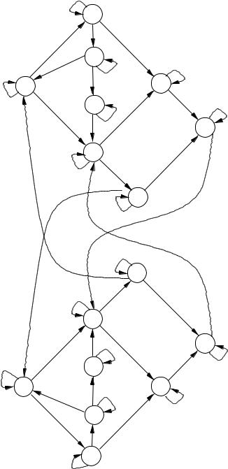
The transition system corresponding to this program is shown in Figure 3.11. Each state shows the values of the variables; for example, ct1 is the state in which process 1 and 2 are critical and trying, respectively, and turn=1. The labels on the transitions show which process was selected for execution. In general, each state has several transitions, some in which process 1 moves and others in which process 2 moves.

This model is a bit di erent from the previous model given for mutual exclusion in Figure 3.8, for these two reasons:

Because the boolean variable turn has been explicitly introduced to distinguish between states s3 and s9 of Figure 3.8, we now distinguish between certain states

Figure 3.11. The transition system corresponding to the SMV code in Figure 3.10. The labels on the transitions denote the process which makes the move. The label 1, 2 means that either process could make that move.