the first time and the result remembered for future calls. This programming technique is known as memoisation. As well as being more e cient, it has the advantage that the resulting OBDD requires less reduction. (In this example, using memoisation eliminates the need for the final call to reduce altogether.) Without memoisation, apply is exponential in the size of its arguments, since each non-leaf call generates a further two calls. With memoisation, the number of calls to apply is bounded by 2 · |Bf | · |Bg |, where |B| is the size of the BDD. This is a worst-time complexity; the actual performance is often much better than this.

6.2.3 The algorithm restrict

Given an OBDD Bf representing a boolean formula f , we need an algorithm restrict such that the call restrict(0, x, Bf ) computes the reduced OBDD representing f [0/x] using the same variable ordering as Bf . The algorithm for restrict(0, x, Bf ) works as follows. For each node n labelled with x, incoming edges are redirected to lo(n) and n is removed. Then we call reduce on the resulting OBDD. The call restrict (1, x, Bf ) proceeds similarly, only we now redirect incoming edges to hi(n).

6.2.4 The algorithm exists

A boolean function can be thought of as putting a constraint on the values of its argument variables. For example, the function x + (y · z) evaluates to 1 only if x is 1; or y is 0 and z is 1 – this is a constraint on x, y, and z.

It is useful to be able to express the relaxation of the constraint on a subset of the variables concerned. To allow this, we write x. f for the boolean function f with the constraint on x relaxed. Formally, x. f is defined as f [0/x] + f [1/x]; that is, x. f is true if f could be made true by putting x

def

to 0 or to 1. Given that x. f = f [0/x] + f [1/x] the exists algorithm can be implemented in terms of the algorithms apply and restrict as

def

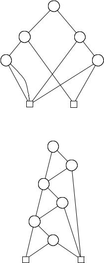
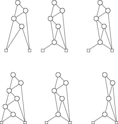
Consider, for example, the OBDD Bf for the function f = x1 · y1 + x2 · y2 + x3 · y3, shown in Figure 6.19. Figure 6.20 shows restrict(0, x3, Bf ) and restrict(1, x3, Bf ) and the result of applying + to them. (In this case the apply function happens to return its second argument.)

We can improve the e ciency of this algorithm. Consider what happens during the apply stage of (6.3). In that case, the apply algorithm works on two BDDs which are identical all the way down to the level of the x-nodes;

0 1

Figure 6.18. An example of a BDD which is not a read-1-BDD.

Figure 6.19. A BDD Bf to illustrate the exists algorithm.

therefore the returned BDD also has that structure down to the x-nodes. At the x-nodes, the two argument BDDs di er, so the apply algorithm will compute the apply of + to these two subBDDs and return that as the subBDD of the result. This is illustrated in Figure 6.20. Therefore, we can compute the OBDD for x. f by taking the OBDD for f and replacing each node labelled with x by the result of calling apply on + and its two branches.

This can easily be generalised to a sequence of exists operations. We write xˆ. f to mean x1. x2. . . . xn. f , where xˆ denotes (x1, x2, . . . , xn).

Figure 6.22. Translating boolean formulas f to OBDDs Bf , given a fixed, global ordering on boolean variables.

Figure 6.23. Upper bounds in terms of the input OBDD(s) for the worst-case running times of our algorithms needed in our implementation of boolean formulas.

6.2.5 Assessment of OBDDs

Time complexities for computing OBDDs We can measure the complexity of the algorithms of the preceding section by giving upper bounds for the running time in terms of the sizes of the input OBDDs. The table in Figure 6.23 summarises these upper bounds (some of those upper bounds may require more sophisticated versions of the algorithms than the versions presented in this chapter). All the operations except nested boolean quantification are practically e cient in the size of the participating OBDDs. Thus, modelling very large systems with this approach will work if the OBDDs