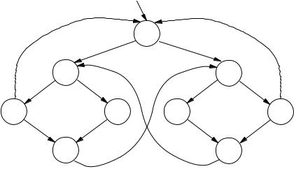
Figure 3.8. A second-attempt model for mutual exclusion. There are now two states representing t1t2, namely s3 and s9.

3.3.2 The NuSMV model checker

So far, this chapter has been quite theoretical; and the sections after this one continue in this vein. However, one of the exciting things about model checking is that it is also a practical subject, for there are several e cient implementations which can check large systems in realistic time. In this section, we look at the NuSMV model-checking system. NuSMV stands for ‘New Symbolic Model Verifier.’ NuSMV is an Open Source product, is actively supported and has a substantial user community. For details on how to obtain it, see the bibliographic notes at the end of the chapter.

NuSMV (sometimes called simply SMV) provides a language for describing the models we have been drawing as diagrams and it directly checks the validity of LTL (and also CTL) formulas on those models. SMV takes as input a text consisting of a program describing a model and some specifications (temporal logic formulas). It produces as output either the word ‘true’ if the specifications hold, or a trace showing why the specification is false for the model represented by our program.

SMV programs consist of one or more modules. As in the programming language C, or Java, one of the modules must be called main. Modules can declare variables and assign to them. Assignments usually give the initial value of a variable and its next value as an expression in terms of the current values of variables. This expression can be non-deterministic (denoted by several expressions in braces, or no assignment at all). Non-determinism is used to model the environment and for abstraction.

192 3 Verification by model checking

The following input to SMV:

MODULE main

VAR

request : boolean; status : {ready,busy};

ASSIGN

init(status) := ready; next(status) := case

request : busy; 1 : {ready,busy};

esac;

LTLSPEC

G(request -> F status=busy)

consists of a program and a specification. The program has two variables, request of type boolean and status of enumeration type {ready, busy}:

0 denotes ‘false’ and 1 represents ‘true.’ The initial and subsequent values of variable request are not determined within this program; this conservatively models that these values are determined by an external environment. This under-specification of request implies that the value of variable status is partially determined: initially, it is ready; and it becomes busy whenever request is true. If request is false, the next value of status is not determined.

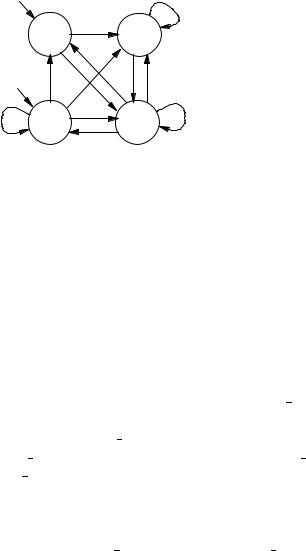
Note that the case 1: signifies the default case, and that case statements are evaluated from the top down: if several expressions to the left of a ‘:’ are true, then the command corresponding to the first, top-most true expression will be executed. The program therefore denotes the transition system shown in Figure 3.9; there are four states, each one corresponding to a possible value of the two binary variables. Note that we wrote ‘busy’ as a shorthand for ‘status=busy’ and ‘req’ for ‘request is true.’

It takes a while to get used to the syntax of SMV and its meaning. Since variable request functions as a genuine environment in this model, the program and the transition system are non-deterministic: i.e., the ‘next state’ is not uniquely defined. Any state transition based on the behaviour of status comes in a pair: to a successor state where request is false, or true, respectively. For example, the state ‘¬req, busy’ has four states it can move to (itself and three others).

LTL specifications are introduced by the keyword LTLSPEC and are simply LTL formulas. Notice that SMV uses &, |, -> and ! for , , → and ¬, respectively, since they are available on standard keyboards. We may

Figure 3.9. The model corresponding to the SMV program in the text.

easily verify that the specification of our module main holds of the model in Figure 3.9.

Modules in SMV SMV supports breaking a system description into several modules, to aid readability and to verify interaction properties. A module is instantiated when a variable having that module name as its type is declared. This defines a set of variables, one for each one declared in the module description. In the example below, which is one of the ones distributed with SMV, a counter which repeatedly counts from 000 through to 111 is described by three single-bit counters. The module counter cell is instantiated three times, with the names bit0, bit1 and bit2. The counter module has one formal parameter, carry in, which is given the actual value 1 in bit0, and bit0.carry out in the instance bit1. Hence, the carry in of module bit1 is the carry out of module bit0. Note that we use the period ‘.’ in m.v to access the variable v in module m. This notation is also used by Alloy (see Chapter 2) and a host of programming languages to access fields in record structures, or methods in objects. The keyword DEFINE is used to assign the expression value & carry in to the symbol carry out (such definitions are just a means for referring to the current value of a certain expression).

MODULE main

VAR

bit0 : counter_cell(1);

bit1 : counter_cell(bit0.carry_out); bit2 : counter_cell(bit1.carry_out);

LTLSPEC

G F bit2.carry_out