Handbook_of_statistical_analysis_using_SAS

Mathematically, correspondence analysis can be regarded as either:

A method for decomposing the chi-squared statistic for a contingency table into components corresponding to different dimensions of the heterogeneity between its rows and columns, or

A method for simultaneously assigning a scale to rows and a separate scale to columns so as to maximize the correlation between the resulting pair of variables.

Quintessentially, however, correspondence analysis is a technique for displaying multivariate categorical data graphically, by deriving coordinate values to represent the categories of the variables involved, which can then be plotted to provide a “picture” of the data.

In the case of two categorical variables forming a two-dimensional contingency table, the required coordinates are obtained from the singular value decomposition (Everitt and Dunn [2001]) of a matrix E with elements eij given by:

where pij = nij /n with nij being the number of observations in the ijth cell of the contingency table and n the total number of observations. The total number of observations in row i is represented by ni+ and the

corresponding value for column j is n . Finally p = ni+ and p = n+j . The

+j i+ ------ +j ------

n n

elements of E can be written in terms of the familiar “observed” (O) and “expected” (E) nomenclature used for contingency tables as:

Written in this way, it is clear that the terms are a form of residual from fitting the independence model to the data.

The singular value decomposition of E consists of finding matrices U, V, and ∆ (diagonal) such that:

where U contains the eigenvectors of EE ′ and V the eigenvectors of E′E. The diagonal matrix ∆ contains the ranked singular values δ k so that δ k2 are the eigenvalues (in decreasing) order of either EE ′ or E′E.

©2002 CRC Press LLC

The coordinate of the ith row category on the kth coordinate axis is given by δ kuik / pi+ , and the coordinate of the jth column category on

the same axis is given by δ kvjk / p+j , where uik, i = 1 … r and vjk, j = 1 … c are, respectively, the elements of the kth column of U and the kth

column of V.

To represent the table fully requires at most R = min(r, c) – 1 dimensions, where r and c are the number of rows and columns of the

where X2 is the usual chi-squared test statistic for independence. In the context of correspondence analysis, X2/n is known as inertia. Correspondence analysis produces a graphical display of the contingency table from the columns of U and V, in most cases from the first two columns, u1, u2, v1, v2, of each, since these give the “best” two-dimensional representation. It can be shown that the first two coordinates give the following approximation to the eij:

so that a large positive residual corresponds to uik and vjk for k = 1 or 2, being large and of the same sign. A large negative residual corresponds to uik and vjk, being large and of opposite sign for each value of k. When uik and vjk are small and their signs are not consistent for each k, the corresponding residual term will be small. The adequacy of the representation produced by the first two coordinates can be informally assessed by calculating the percentages of the inertia they account for; that is

R

∑ δ 2k

k = 1

Values of 60% and above usually mean that the two-dimensional solution gives a reasonable account of the structure in the table.

©2002 CRC Press LLC

16.3Analysis Using SAS

16.3.1 Boyfriends

Assuming that the 15 cell counts shown in Display 16.1 are in an ASCII file, tab separated, a suitable data set can be created as follows:

data boyfriends;

infile 'n:\handbook2\datasets\boyfriends.dat' expandtabs; input c1-c5;

if _n_=1 then rowid='NoBoy'; if _n_=2 then rowid='NoSex'; if _n_=3 then rowid='Both';

label c1='under 16' c2='16-17' c3='17-18' c4='18-19' c5='19-20';

run;

The data are already in the form of a contingency table and can be simply read into a set of variables representing the columns of the table. The label statement is used to assign informative labels to these variables. More informative variable names could also have been used, but labels are more flexible in that they may begin with numbers and include spaces. It is also useful to label the rows, and here the SAS automatic variable _n_ is used to set the values of a character variable rowid.

A correspondence analysis of this table can be performed as follows:

proc corresp data=boyfriends out=coor; var c1-c5;

id rowid; run;

The out= option names the data set that will contain the coordinates of the solution. By default, two dimensions are used and the dimens= option is used to specify an alternative.

The var statement specifies the variables that represent the columns of the contingency table, and the id statement specifies a variable to be used to label the rows. The latter is optional, but without it the rows will simply be labelled row1, row2, etc. The output appears in Display 16.4.

©2002 CRC Press LLC

Degrees of Freedom = 8

Row Coordinates

Summary Statistics for the Row Points

Partial Contributions to Inertia for the Row Points

Indices of the Coordinates that Contribute Most to Inertia for the Row Points

©2002 CRC Press LLC

Squared Cosines for the Row Points

Column Coordinates

The CORRESP Procedure

Summary Statistics for the Column Points

Partial Contributions to Inertia for the Column Points

©2002 CRC Press LLC

Indices of the Coordinates that Contribute Most to Inertia for the Column Points

Squared Cosines for the Column Points

Display 16.4

To produce a plot of the results, a built-in SAS macro, plotit, can be used:

%plotit(data=coor,datatype=corresp,color=black,colors=black);

The resulting plot is shown in Display 16.5. Displaying the categories of a contingency table in a scatterplot in this way involves the concept of distance between the percentage profiles of row or column categories. The distance measure used in a correspondence analysis is known as the chi-squared distance. The calculation of this distance can be illustrated using the proportions of girls in age groups 1 and 2 for each relationship type in Display 16.1.

This is similar to ordinary “straight line” or Pythagorean distance, but differs by dividing each term by the corresponding average proportion.

©2002 CRC Press LLC

In this way, the procedure effectively compensates for the different levels of occurrence of the categories. (More formally, the chance of the chisquared distance for measuring relationships between profiles can be justified as a way of standardizing variables under a multinomial or Poisson distributional assumption; see Greenacre [1992].)

The complete set of chi-squared distances for all pairs of the five age groups, calculated as shown above, can be arranged in a matrix as follows:

The points representing the age groups in Display 16.5 give the twodimensional representation of these distances, the Euclidean distance, between two points representing the chi-square distance between the corresponding age groups. (Similarly for the point representing type of relationship.) For a contingency table with r rows and c columns, it can be shown that the chi-squared distances can be represented exactly in min{r – 1, c – 1} dimensions; here, since r = 3 and c = 5, this means that the coordinates in Display 16.5 will lead to Euclidean distances that are identical to the chi-squared distances given above. For example, the correspondence analysis coordinates for age groups 1 and 2 taken from Display 16.4 are

The corresponding Euclidean distance is calculated as:

( – 0.355 + 0.290) 2 + ( – 0.055 – 0.000) 2

that is, a value of 0.09 — agreeing with the chi-squared distance between the two age groups given previously (Eq. (16.7).

Of most interest in correspondence analysis solutions such as that graphed in Display 16.5 is the joint interpretation of the points representing

©2002 CRC Press LLC

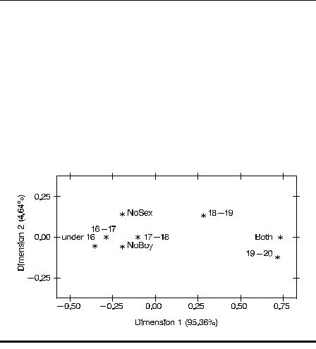
the row and column categories. It can be shown that row and column coordinates that are large and of the same sign correspond to a large positive residual term in the contingency table. Row and column coordinates that are large but of opposite signs imply a cell in the table with a large negative residual. Finally, small coordinate values close to the origin correspond to small residuals. In Display 16.5, for example, age group 5 and boyfriend/sexual intercourse both have large positive coordinate values on the first dimension. Consequently, the corresponding cell in the table will have a large positive residual. Again, age group 5 and boyfriend/no sexual intercourse have coordinate values with opposite signs on both dimensions, implying a negative residual for the corresponding cell in the table.

Display 16.5

16.3.2Smoking and Motherhood

Assuming the cell counts of Display 16.2 are in an ASCII file births.dat and tab separated, they may be read in as follows:

data births;

infile 'n:\handbook2\datasets\births.dat' expandtabs; input c1-c4;

length rowid $12.; select(_n_);

when(1) rowid='Young NS'; when(2) rowid='Young Smoker';

©2002 CRC Press LLC

when(3) rowid='Old NS'; when(4) rowid='Old Smoker';

end;

label c1='Prem Died' c2='Prem Alive' c3='FT Died' c4='FT Alive';

run;

As with the previous example, the data are read into a set of variables corresponding to the columns of the contingency table, and labels assigned to them. The character variable rowid is assigned appropriate values, using the automatic SAS variable _n_ to label the rows. This is explicitly declared as a 12-character variable with the length statement. Where a character variable is assigned values as part of the data step, rather than reading them from a data file, the default length is determined from its first occurrence. In this example, that would have been from rowid='Young NS'; and its length would have been 8 with longer values truncated. This example also shows the use of the select group as an alternative to multiple if-then statements. The expression in parentheses in the select statement is compared to those in the when statements and the rowid variable set accordingly. The end statement terminates the select group.

The correspondence analysis and plot are produced in the same way as for the first example. The output is shown in Display 16.6 and the plot in Display 16.7.

proc corresp data=births out=coor; var c1-c4;

id rowid; run;

%plotit(data=coor,datatype=corresp,color=black,colors=black);

Degrees of Freedom = 9

©2002 CRC Press LLC

Summary Statistics for the Row Points

Partial Contributions to Inertia for the Row Points

Indices of the Coordinates that Contribute Most to Inertia for the Row Points

Squared Cosines for the Row Points

©2002 CRC Press LLC