Data-Structures-And-Algorithms-Alfred-V-Aho

Data Structures and Algorithms: CHAPTER 8: Sorting

pivot) larger then the right groups.

Let us develop a formula for the probability that the left group has i of the n elements, on the assumption that all elements are unequal. For the left group to have i elements, the pivot must be the i + 1st among the n. The pivot, by our method of selection, could either have been in the first position, with one of the i smaller elements second, or it could have been second, with one of the i smaller ones first. The probability that any particular element, such as the i + 1st, appears first in a random order is 1/n. Given that it did appear first, the probability that the second element is one of the i smaller elements out of the n -1 remaining elements is i/(n - 1). Thus the probability that the pivot appears in the first position and is number i + 1 out of n in the proper order is i/n(n - 1). Similarly, the probability that the pivot appears in the second position and is number i + 1 out of n in the sorted order is i/n(n - 1), so the probability that the left group is of size i is 2i/n(n - 1), for 1 ≤ i < n.

Now we can write a recurrence for T(n).

Equation (8.1) says that the average time taken by quicksort is the time, c2n, spent outside of the recursive calls, plus the average time spent in recursive calls. The latter time is expressed in (8.1) as the sum, over all possible i, of the probability that the left group is of size i (and therefore the right group is of size n - i) times the cost of the two recursive calls: T(i) and T(n - i), respectively.

Our first task is to transform (8.1) so that the sum is simplified, and in fact, so (8.1) takes on the form it would have had if we had picked a truly random pivot at each step. To make the transformation, observe that for any function f (i) whatsoever, by substituting i for n - i we may prove

By replacing half the left side of (8.2) by the right side, we see

Applying (8.3) to (8.1), with f(i) equal to the expression inside the summation of

http://www.ourstillwaters.org/stillwaters/csteaching/DataStructuresAndAlgorithms/mf1208.htm (16 of 44) [1.7.2001 19:22:21]

Data Structures and Algorithms: CHAPTER 8: Sorting

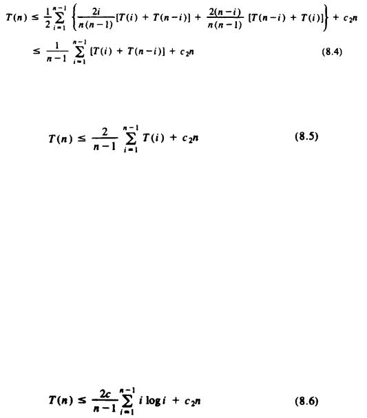
(8.1), we get

Next, we can apply (8.3) to (8.4), with f(i) = T(i). This transformation yields

Note that (8.4) is the recurrence we would get if all sizes between 1 and n - 1 for the left group were equally likely. Thus, picking the larger of two keys as the pivot really doesn't affect the size distribution. We shall study recurrences of this form in greater detail in Chapter 9. Here we shall solve recurrence (8.5) by guessing a solution and showing that it works. The solution we guess is that T(n) £ cn log n for some constant c and all n ³ 2.

To prove that this guess is correct, we perform an induction on n. For n = 2, we have only to observe that for some constant c, T(2) £ 2c log2 = 2c. To prove the induction, assume T(i) £ ci log i for i < n, and substitute this formula for T(i) in the right side of (8.5) to show the resulting quantity is no greater than cn log n. Thus, (8.5) becomes

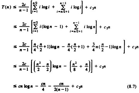
Let us split the summation of (8.6) into low terms, where i £ n/2, and therefore log i is no greater than log(n/2), which is (logn) - 1, and high terms, where i > n/2, and log i may be as large as log n. Then (8.6) becomes

http://www.ourstillwaters.org/stillwaters/csteaching/DataStructuresAndAlgorithms/mf1208.htm (17 of 44) [1.7.2001 19:22:21]

Data Structures and Algorithms: CHAPTER 8: Sorting

If we pick c ³ 4c2, then the sum of the second and fourth terms of (8.7) is no greater than zero. The third term of (8.7) makes a negative contribution, so from (8.7) we may claim that T(n) £ cn log n, if we pick c = 4c2. This completes the proof that quicksort requires O (n log n) time in the average case.

Improvements to Quicksort

Not only is quicksort fast, its average running time is less than that of all other currently known O(n log n) sorting algorithms (by a constant factor, of course). We can improve the constant factor still further if we make some effort to pick pivots that divide each subarray into close-to-equal parts. For example, if we always divide subarrays equally, then each element will be of depth exactly logn, in the tree of partitions analogous to Fig. 8.9. In comparison, the average depth of an element for quicksort as constituted in Fig. 8.14, is about 1.4logn. Thus we could hope to speed up quicksort by choosing pivots carefully.

For example, we could choose three elements of a subarray at random, and pick the middle one as the pivot. We could pick k elements at random for any k, sort them either by a recursive call to quicksort or by one of the simpler sorts of Section 8.2,

and pick the median element, that is, the element, as pivot.† It is an interesting exercise to determine the best value of k, as a function of the number of elements in the subarray to be sorted. If we pick k too small, it costs time because on the average the pivot will divide the elements unequally. If we pick k too large, we spend too much time finding the median of the k elements.

http://www.ourstillwaters.org/stillwaters/csteaching/DataStructuresAndAlgorithms/mf1208.htm (18 of 44) [1.7.2001 19:22:21]

Data Structures and Algorithms: CHAPTER 8: Sorting

Another improvement to quicksort concerns what happens when we get small subarrays. Recall from Section 8.2 that the simple O(n2) methods are better than the O(n log n) methods such as quicksort for small n. How small n is depends on many factors, such as the time spent making a recursive call, which is a property of the machine architecture and the strategy for implementing procedure calls used by the compiler of the language in which the sort is written. Knuth [1973] suggests 9 as the size subarray on which quicksort should call a simpler sorting algorithm.

There is another "speedup" to quicksort that is really a way to trade space for time. The same idea will work for almost any sorting algorithm. If we have the space available, create an array of pointers to the records in array A. We make the comparisons between the keys of records pointed to. But we don't move the records; rather, we move the pointers to records in the same way quicksort moves the records themselves. At the end, the pointers, read in left-to-right order, point to the records in the desired order, and it is then a relatively simple matter to rearrange the records of A into the correct order.

In this manner, we make only n swaps of records, instead of O(n log n) swaps, which makes a substantial difference if records are large. On the negative side, we need extra space for the array of pointers, and accessing keys for comparisons is slower than it was, since we have first to follow a pointer, then go into the record, to get the key field.

8.4 Heapsort

In this section we develop a sorting algorithm called heapsort whose worst case as well as average case running time is O(nlogn). This algorithm can be expressed abstractly using the four set operations INSERT, DELETE, EMPTY, and MIN introduced in Chapters 4 and 5. Suppose L is a list of the elements to be sorted and S a set of elements of type recordtype, which will be used to hold the elements as they are being sorted. The MIN operator applies to the key field of records; that is, MIN(S) returns the record in S with the smallest key value. Figure 8.16 presents the abstract sorting algorithm that we shall transform into heapsort.

(1)for x on list L do

(2)INSERT(x, S);

(3)while not EMPTY(S) do begin

(4)y := MIN(S);

(5)writeln(y);

(6)DELETE(y, S)

end

http://www.ourstillwaters.org/stillwaters/csteaching/DataStructuresAndAlgorithms/mf1208.htm (19 of 44) [1.7.2001 19:22:21]

Data Structures and Algorithms: CHAPTER 8: Sorting

Fig. 8.16. An abstract sorting algorithm.

In Chapters 4 and 5 we presented several data structures, such as 2-3 trees, capable of supporting each of these set operations in O(logn) time per operation, if sets never grow beyond n elements. If we assume list L is of length n, then the number of operations performed is n INSERT's, n MIN's, n DELETE's, and n + 1 EMPTY tests. The total time spent by the algorithm of Fig. 8.16 is thus O(nlogn), if a suitable data structure is used.

The partially ordered tree data structure introduced in Section 4.11 is well suited for the implementation of this algorithm. Recall that a partially ordered tree can be represented by a heap, an array A[1], . . . , A[n], whose elements have the partially ordered tree property: A[i].key £ A[2*i].key and A[i].key £ A[2*i + 1].key. If we think of the elements at 2i and 2i + 1 as the "children" of the element at i, then the array forms a balanced binary tree in which the key of the parent never exceeds the keys of the children.

We showed in Section 4.11 that the partially ordered tree could support the operations INSERT and DELETEMIN in O(logn) time per operation. While the partially ordered tree cannot support the general DELETE operation in O(logn) time (just finding an arbitrary element takes linear time in the worst case), we should notice that in Fig. 8.16 the only elements we delete are the ones found to be minimal. Thus lines (4) and (6) of Fig. 8.16 can be combined into a DELETEMIN function that returns the element y. We can thus implement Fig. 8.16 using the partially ordered tree data structure of Section 4.11.

We shall make one more modification to the algorithm of Fig. 8.16 to avoid having to print the elements as we delete them. The set S will always be stored as a heap in the top of array A, as A[1], . . . , A[i], if S has i elements. By the partially ordered tree property, the smallest element is always in A[1]. The elements already deleted from S can be stored in A [i + 1], . . . ,A [n], sorted in reverse order, that is, with A[i + 1] ³ A[i + 2]³ × × × ³ A[n].† Since A[1] must be smallest among A[1], . . . , A[i], we may effect the DELETEMIN operation by simply swapping A[1] with A[i]. Since the new A[i] (the old A[1]) is no smaller than A[i + 1] (or else the former would have been deleted from S before the latter), we now have A[i], . . . , A[n] sorted in decreasing order. We may now regard S as occupying A[1], . . . ,A [i - 1].

Since the new A[1] (old A[i]) violates the partially ordered tree property, we must push it down the tree as in the procedure DELETEMIN of Fig. 4.23. Here, we use the procedure pushdown shown in Fig. 8.17 that operates on the externally defined array A. By a sequence of swaps, pushdown pushes element A[first] down through its

http://www.ourstillwaters.org/stillwaters/csteaching/DataStructuresAndAlgorithms/mf1208.htm (20 of 44) [1.7.2001 19:22:21]

Data Structures and Algorithms: CHAPTER 8: Sorting

descendants to its proper position in the tree. To restore the partially ordered tree property to the heap, we call pushdown with first = 1.

We now see how lines (4 - 6) of Fig. 8.16 are to be done. Selecting the minimum at line (4) is easy; it is always in A[l] because of the partially ordered tree property. Instead of printing at line (5), we swap A[1] with A[i], the last element in the current heap. Deleting the minimum element from the partially ordered tree is now easy; we just decrement i, the cursor that indicates the end of the current heap. We then invoke pushdown(1, i) to restore the partially ordered tree property to the heap A[1], . . . , A[i].

The test for emptiness of S at line (3) of Fig. 8.16 is done by testing the value of i, the cursor marking the end of the current heap. Now we have only to consider how to perform lines (1) and (2). We may assume L is originally present in A[1], . . . , A[n] in some order. To establish the partially ordered tree property initially, we call pushdown(j,n) for all j = n/2, n/2 - 1 , . . . , 1. We observe that after calling pushdown(j, n), no violations of the partially ordered tree property occur in A[j], . . . , A[n] because pushing a record down the tree does not introduce new violations, since we only swap a violating record with its smaller child. The complete procedure, called heapsort, is shown in Fig. 8.18.

Analysis of Heapsort

Let us examine the procedure pushdown to see how long it takes. An inspection of Fig. 8.17 confirms that the body of the while-loop takes constant time. Also, after each iteration, r has at least twice the value it had before. Thus, since r starts off equal to first, after i iterations we have r ³ first * 2i.

procedure pushdown ( first, last: integer );

{assumes A[first], . . . ,A[last] obeys partially ordered tree property except possibly for the children of A[first]. The procedure pushes A[first] down until the partially ordered tree property is restored }

var

r: integer; { indicates the current position of A[first] } begin

r := first; { initialization } while r < = last div 2 do

if last = 2*r then begin { r has one child at 2*r } if A[r].key > A[2*r].key

then

swap(A[r], A[2*r]);

http://www.ourstillwaters.org/stillwaters/csteaching/DataStructuresAndAlgorithms/mf1208.htm (21 of 44) [1.7.2001 19:22:21]

Data Structures and Algorithms: CHAPTER 8: Sorting

r := last { forces a break from the while-loop } end

else { r has two children, elements at 2*r and 2*r + 1 } if A[r].key > A[2*r].key

and

A[2*r].key < = A[2*r + l].key then

begin

{ swap r with left child } swap(A[r], A[2*r]);

r := 2*r

end

else if A[r].key > A[2*r + l].key

and

A[2*r + l].key < A[2*r].key then

begin

{ swap r with right child } swap(A[r], A[2*r + 1]);

r := 2*r + l

end

else { r does not violate partially ordered tree property } r := last { to break while-loop }

end; { pushdown }

Fig. 8.17. The procedure pushdown.

Surely, r > last/2 if first * 2i > last/2, that is if

Hence, the number of iterations of the while-loop of pushdown is at most log(last/first).

Since first ³ 1 and last £ n in each call to pushdown by the heapsort algorithm of Fig. 8.18, (8.8) says that each call to pushdown, at line (2) or (5) of Fig. 8.18, takes O(logn) time. Clearly the loop of lines (1) and (2) iterates n/2 times, so the time spent in lines (1 - 2) is O(n logn).† Also, the loop of

procedure heapsort;

{ sorts array A[1], . . . ,A[n] into decreasing order } var

http://www.ourstillwaters.org/stillwaters/csteaching/DataStructuresAndAlgorithms/mf1208.htm (22 of 44) [1.7.2001 19:22:21]

Data Structures and Algorithms: CHAPTER 8: Sorting

i: integer; { cursor into A } begin

{establish the partially ordered tree property initially }

(1)for i := n div 2 downto 1 do

(2) pushdown(i, n );

(3)for i := n downto 2 do begin

{ re-establish partially ordered tree property }

end

end; { heapsort }

Fig. 8.18. The procedure heapsort.

lines (3 - 5) iterates n - 1 times. Thus, a total of O(n) time is spent in all repetitions of swap at line (4), and O (n log n) time is spent during all repetitions of line (5). Hence, the total time spent in the loop of lines (3 - 5) is O (n log n ), and all of heapsort takes O (n log n) time.

Despite its O (n log n) worst case time, heapsort will, on the average take more time than quicksort, by a small constant factor. Heapsort is of intellectual interest, because it is the first O(n log n) worst-case sort we have covered. It is of practical utility in the situation where we want not all n elements sorted, but only the smallest k of them for some k much less than n. As we mentioned, lines (1 - 2) really take only O(n) time. If we make only k iterations of lines (3 - 5), the time spent in that loop is O(k log n). Thus, heapsort, modified to produce only the first k elements takes O(n + k log n) time. If k ≤ n/log n, that is, we want at most (1/log n)th of the entire sorted list, then the required time is O(n).

8.5 Bin Sorting

One might wonder whether Ω (n log n) steps are necessary to sort n elements. In the next section, we shall show that to be the case for sorting algorithms that assume nothing about the data type of keys, except that they can be ordered by some function that tells whether one key value is "less than" another. We can often sort in less than O(n log n) time, however, when we know something special about the keys being sorted.

Example 8.5. Suppose keytype is integer, and the values of the key are known to be in the range l to n, with no duplicates, where n is the number of elements. Then if A

http://www.ourstillwaters.org/stillwaters/csteaching/DataStructuresAndAlgorithms/mf1208.htm (23 of 44) [1.7.2001 19:22:21]

Data Structures and Algorithms: CHAPTER 8: Sorting

and B are of type array[1..n] of recordtype, and the n elements to be sorted are initially in A, we can place them in the array B, in order of their keys by

This code calculates where record A[i] belongs and places it there. The entire loop takes O(n) time. It works correctly only when there is exactly one record with key v for each value of v between 1 and n. A second record with key value v would also be placed in B[v], obliterating the previous record with key v.

There are other ways to sort an array A with keys 1,2, . . . , n in place in only O(n) time. Visit A[1], . . . , A[n] in turn. If the record in A[i] has key j ¹ i, swap A[i] with A[j]. If, after swapping, the record with key k is now in A[i], and k ¹ i, swap A[i] with A[k], and so on. Each swap places some record where it belongs, and once a record is where it belongs, it is never moved. Thus, the following algorithm sorts A in place, in O(n) time, provided there is one record with each of keys 1, 2 , . . . , n.

for i := 1 to n do

while A [i].key < > i do swap(A[i], A[A[i].key]);

The program (8.9) given in Example 8.5 is a simple example of a "binsort," a sorting process where we create a "bin" to hold all the records with a certain key value. We examine each record r to be sorted and place it in the bin for the key value of r. In the program (8.9) the bins are the array elements B[1], . . . , B[n], and B[i] is the bin for key value i. We can use array elements as bins in this simple case, because we know we never put more than one record in a bin. Moreover, we need not assemble the bins into a sorted list here, because B serves as such a list.

In the general case, however, we must be prepared both to store more than one record in a bin and to string the bins together (or concatenate) the bins in proper order. To be specific, suppose that, as always, A[1], . . . , A[n] is an array of type recordtype, and that the keys for records are of type keytype. Suppose for the purposes of this section only, that keytype is an enumerated type, such as l..m or char. Let listtype be a type that represents lists of elements of type recordtype; listtype could be any of the types for lists mentioned in Chapter 2, but a linked list is most effective, since we shall be growing lists of unpredictable size in each bin, yet the total lengths of the lists is fixed at n, and therefore an array of n cells can supply the lists for the various bins as needed.

http://www.ourstillwaters.org/stillwaters/csteaching/DataStructuresAndAlgorithms/mf1208.htm (24 of 44) [1.7.2001 19:22:21]

Data Structures and Algorithms: CHAPTER 8: Sorting

Finally, let B be an array of type array[keytype] of listtype. Thus, B is an array of bins, which are lists (or, if the linked list representation is used, headers for lists). B is indexed by keytype, so there is one bin for each possible key value. In this manner we can effect the first generalization of (8.9) -- the bins have arbitrary capacity.

Now we must consider how the bins are to be concatenated. Abstractly, we must form from lists a1, a2, . . . ,ai and b1, b2, . . . , bj the concatenation of the lists, which is a1, a2, . . . ,ai. b1, b2, . . . ,bj. The implementation of this operation CONCATENATE(L1, L2), which replaces list L1 by the concatenation L1L2, can be done in any of the list representations we studied in Chapter 2.

For efficiency, however, it is useful to have, in addition to a header, a pointer to the last element on each list (or to the header if the list is empty). This modification facilitates finding the last element on list L1 without running down the entire list.

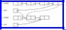
Figure 8.19 shows, by dashed lines, the revised pointers necessary to concatenate L1 and L2 and to have the result be called L1. List L1 is assumed to "disappear" after concatenation, in the sense that the header and end pointer for L2 become null.

Fig. 8.19. Concatenation of linked lists.

We can now write a program to binsort arbitrary collections of records, where the key field is of an enumerated type. The program, shown in Fig. 8.20, is written in terms of list processing primitives. As we mentioned, a linked list is the preferred implementation, but options exist. Recall also that the setting for the procedure is that an array A of type array[1..n] of recordtype holds the elements to be sorted, and array B, of type array [keytype] of listtype represents the bins. We assume keytype is expressible as lowkey..highkey, as any enumerated type must be, for some quantities lowkey and highkey.

procedure binsort;

{ binsort array A, leaving the sorted list in B[lowkey] } var

i: integer; v: keytype;

begin

{ place the records into bins }

http://www.ourstillwaters.org/stillwaters/csteaching/DataStructuresAndAlgorithms/mf1208.htm (25 of 44) [1.7.2001 19:22:21]