Data-Structures-And-Algorithms-Alfred-V-Aho

Data Structures and Algorithms: CHAPTER 9: Algorithm Analysis Techniques

Secondly we have not yet determined the exact asymptotic growth rate for f(n), although we have shown that it is no worse than O(nlogn). If we guess a slower growing solution, like f(n) = an, or f(n) = anloglogn, we cannot prove the claim that T(n) £ f(n). However, the matter can only be settled conclusively by examining mergesort and showing that it really does take W(nlogn) time; in fact, it takes time proportional to nlogn on all inputs, not just on the worst possible inputs. We leave this observation as an exercise.

Example 9.1 exposes a general technique for proving some function to be an upper bound on the running time of an algorithm. Suppose we are given the recurrence equation

Note that (9.5) generalizes (9.1), where g(x, y) is 2x + c2y. Also observe that we could imagine equations more general than (9.5). For example, the formula g might involve all of T(n-1), T(n-2), . . . , T(1), not just T(n/2). Also, we might be given values for T(1), T(2), . . . , T(k), and the recurrence would then apply only for n > k. The reader can, as an exercise, consider how to solve these more general recurrences by method (1) -- guessing a solution and verifying it.

Let us turn our attention to (9.5) rather than its generalizations. Suppose we guess a function f(a1, . . . , aj, n), where a1, . . . , aj are parameters, and attempt to prove by

induction on n that T(n) £ f(a1, . . . , aj, n). For example, our guess in Example 9.1 was f(a1, a2, n) = a1nlogn + a2, but we used a and b for a1 and a2. To check that for some values of a1, . . . , aj we have T(n) £ f(a1, . . . , aj, n) for all n ³ 1, we must satisfy

f(a1, . . . , aj, 1) ³ c

f(a1, . . . , aj, n) ³ g(f(a1, . . . , aj, n/2), n) (9.6)

http://www.ourstillwaters.org/stillwaters/csteaching/DataStructuresAndAlgorithms/mf1209.htm (6 of 19) [1.7.2001 19:24:52]

Data Structures and Algorithms: CHAPTER 9: Algorithm Analysis Techniques

That is, by the inductive hypothesis, we may substitute f for T on the right side of the recurrence (9.5) to get

T(n) ≤

g(f(a1, . . . , aj, n/2), n) (9.7)

When the second line of (9.6) holds, we can combine it with (9.7) to prove that T(n) ≤ f(a1, . . . , an, n), which is what we wanted to prove by induction on n.

For example, in Example 9.1, we have g(x, y) = 2x + c2y and f(a1, a2, n) = a1nlogn + a2. Here we must try to satisfy

As we discussed, a2 = c1 and a1 = c1 + c2 is a satisfactory choice.

Expanding Recurrences

If we cannot guess a solution, or we are not sure we have the best bound on T(n), we can use a method that in principle always succeeds in solving for T(n) exactly, although in practice we often have trouble summing series and must resort to computing an upper bound on the sum. The general idea is to take a recurrence like (9.1), which says T(n) ≤ 2T(n/2) + c2n, and use it to get a bound on T(n/2) by substituting n/2 for n. That is

T(n/2) ≤ 2T(n/4) + c2n/2 (9.8)

Substituting the right side of (9.8) for T(n/2) in (9.1) yields

http://www.ourstillwaters.org/stillwaters/csteaching/DataStructuresAndAlgorithms/mf1209.htm (7 of 19) [1.7.2001 19:24:52]

Data Structures and Algorithms: CHAPTER 9: Algorithm Analysis Techniques

T(n) ≤ 2(2T(n/4) + c2n/2) + c2n = 4T(n/4) + 2c2n (9.9)

Similarly, we could substitute n/4 for n in (9.1) and use it to get a bound on T(n/4). That bound, which is 2T(n/8) + c2n/4, can be substituted in the right of (9.9) to yield

Now the reader should perceive a pattern. By induction on i we can obtain the relationship

T(n) ≤

2iT(n/2i)+ic2n (9.11)

for any i. Assuming n is a power of 2, say 2k, this expansion process comes to a halt as soon as we get T(1) on the right of (9.11). That will occur when i = k, whereupon (9.11) becomes

T(n) ≤ 2kT(1) + kc2n

(9.12)

Then, since 2k = n, we know k = logn. As T(1) ≤ c1, (9.12) becomes

T(n) ≤ c1n + c2nlogn

(9.13)

Equation (9.13) is actually as tight a bound as we can put on T(n), and proves that

http://www.ourstillwaters.org/stillwaters/csteaching/DataStructuresAndAlgorithms/mf1209.htm (8 of 19) [1.7.2001 19:24:52]

Data Structures and Algorithms: CHAPTER 9: Algorithm Analysis Techniques

T(n) is O(nlogn).

9.4 A General Solution for a Large Class of Recurrences

Consider the recurrence that one gets by dividing a problem of size n into a subproblems each of size n/b. For convenience, we assume that a problem of size 1 takes one time unit and that the time to piece together the solutions to the subproblems to make a solution for the size n problem is d(n), in the same time units. For our mergesort example, we have a = b = 2, and d(n) = c2n/c1, in units of c1. Then if T(n) is the time to solve a problem of size n, we have

T(1) = 1

T(n) = aT(n/b) + d(n)

(9.14)

Note that (9.14) only applies to n's that are an integer power of b, but if we assume T(n) is smooth, getting a tight upper bound on T(n) for those values of n tells us how T(n) grows in general.

Also note that we use equality in (9.14) while in (9.1) we had an inequality. The reason is that here d(n) can be arbitrary, and therefore exact, while in (9.1) the assumption that c2n was the worst case time to merge, for one constant c2 and all n, was only an upper bound; the actual worst case running time on inputs of size n may have been less than 2T(n/2) + c2n. Actually, whether we use = or ≤ in the recurrence makes little difference, since we wind up with an upper bound on the worst case running time anyway.

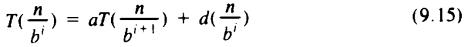
To solve (9.14) we use the technique of repeatedly substituting for T on the right side, as we did for a specific example in our previous discussion of expanding recurrences. That is, substituting n/bi for n in the second line of (9.14) yields

Thus, starting with (9.14) and substituting (9.15) for i = 1, 2, . . . , we get

http://www.ourstillwaters.org/stillwaters/csteaching/DataStructuresAndAlgorithms/mf1209.htm (9 of 19) [1.7.2001 19:24:52]

Data Structures and Algorithms: CHAPTER 9: Algorithm Analysis Techniques

Now, if we assume n = bk, we can use the fact that T(n/bk) = T(1) = 1 to get from the above, with i = k, the formula

If we use the fact that k = logbn, the first term of (9.16) can be written as alogbn , or

equivalently nlogba (take logarithms to the base b of both expressions to see that they are the same). This expression is n to a constant power. For example, in the case of mergesort, where a = b = 2, the first term is n. In general, the larger a is, i.e., the more subproblems we need to solve, the higher the exponent will be; the higher b is, i.e., the smaller each subproblem is, the lower will be the exponent.

Homogeneous and Particular Solutions

It is interesting to see the different roles played by the two terms in (9.16). The first, ak or nlogba, is called the homogeneous solution, in analogy with differential equation terminology. The homogeneous solution is the exact solution when d(n), called the driving function, is 0 for all n. In other words, the homogeneous solution represents the cost of solving all the subproblems, even if subproblems can be combined "for free."

On the other hand, the second term of (9.16) represents the cost of creating the subproblems and combining their results. We call this term the particular solution. The particular solution is affected by both the driving function and the number and size of subproblems. As a rule of thumb if the homogeneous solution is greater than the driving function, then the particular solution has the same growth rate as the homogeneous solution. If the driving function grows faster than the homogeneous solution by more than n for some > 0, then the particular solution has the same

http://www.ourstillwaters.org/stillwaters/csteaching/DataStructuresAndAlgorithms/mf1209.htm (10 of 19) [1.7.2001 19:24:52]

Data Structures and Algorithms: CHAPTER 9: Algorithm Analysis Techniques

growth rate as the driving function. If the driving function has the same growth rate as the homogeneous solution, or grows faster by at most logkn for some k, then the particular solution grows as logn times the driving function.

It is important to recognize that when searching for improvements in an algorithm, we must be alert to whether the homogeneous solution is larger than the driving function. For example, if the homogeneous solution is larger, then finding a faster way to combine subproblems will have essentially no effect on the efficiency of the overall algorithm. What we must do in that case is find a way to divide a problem into fewer or smaller subproblems. That will affect the homogeneous solution and lower the overall running time.

If the driving function exceeds the homogeneous solution, then one must try to decrease the driving function. For example, in the mergesort case, where a = b = 2, and d(n) = cn, we shall see that the particular solution is O(nlogn). However, reducing d(n) to a slightly sublinear function, say n0.9, will, as we shall see, make the particular solution less than linear as well and reduce the overall running time to O(n), which is the homogeneous solution. †

Multiplicative Functions

The particular solution in (9.16) is hard to evaluate, even if we know what d(n) is. However, for certain common functions d(n), we can solve (9.16) exactly, and there are others for which we can get a good upper bound. We say a function f on integers is multiplicative if f(xy) = f(x)f(y) for all positive integers x and y.

Example 9.2. The multiplicative functions that are of greatest interest to us are of the form nα for any positive α. To prove f(n) = nα is multiplicative, we have only to observe that (xy)α = xαyα.

Now if d(n) in (9.16) is multiplicative, then d(bk-j) = (d(b))k-j, and the particular solution of (9.16) is

http://www.ourstillwaters.org/stillwaters/csteaching/DataStructuresAndAlgorithms/mf1209.htm (11 of 19) [1.7.2001 19:24:52]

Data Structures and Algorithms: CHAPTER 9: Algorithm Analysis Techniques

There are three cases to consider, depending on whether a is greater than, less than, or equal to d(b).

1.If a > d(b), then the formula (9.17) is O(ak), which we recall is nlogba, since k = logbn. In this case, the particular and homogeneous solutions are the same,

and depend only on a and b, and not on the driving function d. Thus, improvements in the running time must come from decreasing a or increasing b; decreasing d(n) is of no help.

2.If a < d(b), then (9.17) is O(d(b)k), or equivalently O(nlogbd(b)). In this case, the particular solution exceeds the homogeneous, and we may also look to the

driving function d(n) as well as to a and b, for improvements. Note the important special case where d(n) = nα. Then d(b) = bα, and logb(bα) = α. Thus the particular solution is O(nα), or O(d(n)).

3.If a = d(b), we must reconsider the calculation involved in (9.17), as our formula for the sum of a geometric series is now inappropriate. In this case we have

Since a = d(b), the particular solution given by (9.18) is logbn times the homogeneous solution, and again the particular solution exceeds the homogeneous.

http://www.ourstillwaters.org/stillwaters/csteaching/DataStructuresAndAlgorithms/mf1209.htm (12 of 19) [1.7.2001 19:24:52]

Data Structures and Algorithms: CHAPTER 9: Algorithm Analysis Techniques

In the special case d(n) = nα, (9.18) reduces to O(nαlogn), by observations similar to those in Case (2).

Example 9.3. Consider the following recurrences, with T(1) = 1.

1.T(n) = 4T(n/2) + n

2.T(n) = 4T(n/2) + n2

3.T(n) = 4T(n/2) + n3

In each case, a = 4, b = 2, and the homogeneous solution is n2. In Equation (1), with d(n) = n, we have d(b) = 2. Since a = 4 > d(b), the particular solution is also n2, and T(n) is O(n2) in (1).

In Equation (3), d(n) = n3 d(b) = 8, and a < d(b). Thus the particular solution is O(nlogbd(b)) = O(n3), and T(n) of Equation (3) is O(n3). We can deduce that the particular solution is of the same order as d(n) = n3, using the observations made above about d(n)'s of the form nα in analyzing the case a < d(b) of (9.17). In Equation (2) we have d(b) = 4 = a, so (9.18) applies. As d(n) is of the form nα, the particular solution, and therefore T(n) itself, is O(n2 log n).

Other Driving Functions

These are other functions that are not multiplicative, yet for which we can get solutions for (9.16) or even (9.17). We shall consider two examples. The first generalizes to any function that is the product of a multiplicative function and a constant greater than or equal to one. The second is typical of a case where we must examine (9.16) in detail and get a close upper bound on the particular solution.

Example 9.4. Consider

T(1) = 1

T(n) = 3T(n/2) + 2n1.5

Now 2n1.5 is not multiplicative, but n1.5 is. Let U(n) = T(n)/2 for all n. Then

U(1) = 1/2

http://www.ourstillwaters.org/stillwaters/csteaching/DataStructuresAndAlgorithms/mf1209.htm (13 of 19) [1.7.2001 19:24:52]

Data Structures and Algorithms: CHAPTER 9: Algorithm Analysis Techniques

U(n) = 3U(n/2) + n1.5

The homogeneous solution, if U(1) were 1, would be nlog 3 < n1.59; since U(1) = 1/2 we can easily show the homogeneous solution is less than n1.59/2; certainly it is O(n1.59). For the particular solution, we can ignore the fact that U(1) ¹ 1, since increasing U(1) will surely not lower the particular solution. Then since a = 3, b = 2, and b1.5 = 2.83 < a, the particular solution is also O(n1.59), and that is the growth rate of U(n). Since T(n) = 2U(n), T(n) is also O(n1.59) or O(nlog 3).

Example 9.5. Consider

T(1) = 1

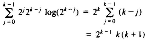
T(n) = 2T(n/2) + n log n

The homogeneous solution is easily seen to be n, since a = b = 2. However, d(n) = n log n is not multiplicative, and we must sum the particular solution formula in (9.16) by ad hoc means. That is, we want to evaluate

Since k = log n we have the particular solution O (n log2n), and this solution, being greater than the homogeneous, is also the value of T(n) that we obtain.

Exercises

http://www.ourstillwaters.org/stillwaters/csteaching/DataStructuresAndAlgorithms/mf1209.htm (14 of 19) [1.7.2001 19:24:52]

Data Structures and Algorithms: CHAPTER 9: Algorithm Analysis Techniques

Write recurrence equations for the time and space complexity of the following algorithm, assuming n is a power of 2.

function path ( s, t, n: integer ) : boolean; begin

if n = 1 then

if edge (s, t) then return (true)

else

return (false);

9.1

{ if we reach here, n > 1 } for i := 1 to n do

if path(s, i, n div 2) and path (i, t, n div 2) then

return (true); return (false)

end; { path }

The function edge(i, j) returns true if vertices i and j of an n-vertex graph are connected by an edge or if i = j; edge(i, j) returns false otherwise. What does the program do?

Solve the following recurrences, where T(1) = 1 and T(n) for n ³ 2 satisfies:

a. T(n) = 3T(n/2) + n

9.2

b.T(n) = 3T(n/2) + n2

c.T(n) = 8T(n/2) + n3

http://www.ourstillwaters.org/stillwaters/csteaching/DataStructuresAndAlgorithms/mf1209.htm (15 of 19) [1.7.2001 19:24:52]