Data-Structures-And-Algorithms-Alfred-V-Aho

Data Structures and Algorithms: CHAPTER 10: Algorithm Design Techniques

Fig. 10.13. A minimal cost triangulation.

10.3 Greedy Algorithms

Consider the problem of making change. Assume coins of values 25¢ (quarter), 10¢ (dime), 5¢ (nickel) and 1¢ (penny), and suppose we want to return 63¢ in change. Almost without thinking we convert this amount to two quarters, one dime and three pennies. Not only were we able to determine quickly a list of coins with the correct value, but we produced the shortest list of coins with that value.

The algorithm the reader probably used was to select the largest coin whose value was not greater than 63¢ (a quarter), add it to the list and subtract its value from 63 getting 38¢. We then selected the largest coin whose value was not greater than 38¢ (another quarter) and added it to the list, and so on.

This method of making change is a greedy algorithm. At any individual stage a greedy algorithm selects that option which is "locally optimal" in some particular sense. Note that the greedy algorithm for making change produces an overall optimal solution only because of special properties of the coins. If the coins had values 1¢, 5¢, and 11¢ and we were to make change of 15¢, the greedy algorithm would first select an 11¢ coin and then four 1¢ coins, for a total of five coins. However, three 5¢ coins would suffice.

We have already seen several greedy algorithms, such as Dijkstra's shortest path algorithm and Kruskal's minimum cost spanning tree algorithm. Dijkstra's shortest path algorithm is "greedy" in the sense that it always chooses the closest vertex to the source among those whose shortest path is not yet known. Kruskal's algorithm is also "greedy"; it picks from the remaining edges the shortest among those that do not create a cycle.

We should emphasize that not every greedy approach succeeds in producing the best result overall. Just as in life, a greedy strategy may produce a good result for a while, yet the overall result may be poor. As an example, we might consider what happens when we allow negative-weight edges in Dijkstra's and Kruskal's algorithms. It turns out that Kruskal's spanning tree algorithm is not affected; it still produces the minimum cost tree. But Dijkstra's algorithm fails to produce shortest paths in some cases.

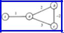
Example 10.4. We see in Fig. 10.14 a graph with a negative cost edge between b and c. If we apply Dijkstra's algorithm with source s, we correctly discover first that the

http://www.ourstillwaters.org/stillwaters/csteaching/DataStructuresAndAlgorithms/mf1210.htm (16 of 40) [1.7.2001 19:27:46]

Data Structures and Algorithms: CHAPTER 10: Algorithm Design Techniques

minimum path to a has length 1. Now, considering only edges from s or a to b or c, we expect that b has the shortest path from s, namely s → a → b, of length 3. We then discover that c has a shortest path from s of length 1.

Fig. 10.14. Graph with negative weight edge.

However, our "greedy" selection of b before c was wrong from a global point of view. It turns out that the path s → a → c → b has length only 2, so our minimum distance of 3 for b was wrong.†

Greedy Algorithms as Heuristics

For some problems no known greedy algorithm produces an optimal solution, yet there are greedy algorithms that can be relied upon to produce "good" solutions with high probability. Frequently, a suboptimal solution with a cost a few percent above optimal is quite satisfactory. In these cases, a greedy algorithm often provides the fastest way to get a "good" solution. In fact, if the problem is such that the only way to get an optimal solution is to use an exhaustive search technique, then a greedy algorithm or other heuristic for getting a good, but not necessarily optimal, solution may be our only real choice.

Example 10.5. Let us introduce a famous problem where the only known algorithms that produce optimal solutions are of the "try-all-possibilities" variety and can have running times that are exponential in the size of the input. The problem, called the traveling salesman problem, or TSP, is to find, in an undirected graph with weights on the edges, a tour (a simple cycle that includes all the vertices) the sum of whose edge-weights is a minimum. A tour is often called a Hamilton (or Hamiltonian) cycle.

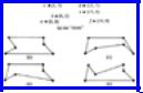
Figure 10.15(a) shows one instance of the traveling salesman problem, a graph with six vertices (often called "cities"). The coordinates of each vertex are given, and we take the weight of each edge to be its length. Note that, as is conventional with the TSP, we assume all edges exist, that is, the graph is complete. In more general instances, where the weight of edges is not based on Euclidean distance, we might find a weight of infinity on an edge that really was not present.

Figure 10.15(b)-(e) shows four tours of the six "cities" of Fig. 10.15(a). The reader might ponder which of these four, if any, is optimal. The lengths of these four tours

http://www.ourstillwaters.org/stillwaters/csteaching/DataStructuresAndAlgorithms/mf1210.htm (17 of 40) [1.7.2001 19:27:46]

Data Structures and Algorithms: CHAPTER 10: Algorithm Design Techniques

are 50.00, 49.73, 48.39, and 49.78, respectively; (d) is the shortest of all possible tours.

Fig. 10.15. An instance of the traveling salesman problem.

The TSP has a number of practical applications. As its name implies, it can be used to route a person who must visit a number of points and return to his starting point. For example, the TSP has been used to route collectors of coins from pay phones.

The vertices are the phones and the "home base." The cost of each edge is the travel time between the two points in question.

Another "application" of the TSP is in solving the knight's tour problem: find a sequence of moves whereby a knight can visit each square of the chessboard exactly once and return to its starting point. Let the vertices be the chessboard squares and let the edges between two squares that are a knight's move apart have weight 0; all other edges have weight infinity. An optimal tour has weight 0 and must be a knight's tour. Surprisingly, good heuristics for the TSP have no trouble finding knight's tours, although finding one "by hand" is a challenge.

The greedy algorithm for the TSP we have in mind is a variant of Kruskal's algorithm. Like that algorithm, we shall consider edges shortest first. In Kruskal's algorithm we accept an edge in its turn if it does not form a cycle with the edges already accepted, and we reject the edge otherwise. For the TSP, the acceptance criterion is that an edge under consideration, together with already selected edges,

1.does not cause a vertex to have degree three or more, and

2.does not form a cycle, unless the number of selected edges equals the number of vertices in the problem.

Collections of edges selected under these criteria will form a collection of unconnected paths, until the last step, when the single remaining path is closed to form a tour.

In Fig. 10.15(a), we would first pick edge (d, e), since it is the shortest, having length 3. Then we consider edges (b, c), (a, b), and (e, f), all of which have length 5. It doesn't matter in which order we consider them; all meet the conditions for selection, and we must select them if we are to follow the greedy approach. Next

http://www.ourstillwaters.org/stillwaters/csteaching/DataStructuresAndAlgorithms/mf1210.htm (18 of 40) [1.7.2001 19:27:46]

Data Structures and Algorithms: CHAPTER 10: Algorithm Design Techniques

shortest edge is (a, c), with length 7.08. However, this edge would form a cycle with (a, b) and (b, c), so we reject it. Edge (d, f) is next rejected on similar grounds. Edge (b, e) is next to be considered, but it must be rejected because it would raise the degrees of b and e to three, and could then never form a tour with what we had selected. Similarly we reject (b, d). Next considered is (c, d), which is accepted. We now have one path, a → b → c → d → e → f, and eventually accept (a, f) to complete the tour. The resulting tour is Fig. 10.15(b), which is fourth best of all the tours, but less than 4% more costly than the optimal.

10.4 Backtracking

Sometimes we are faced with the task of finding an optimal solution to a problem, yet there appears to be no applicable theory to help us find the optimum, except by resorting to exhaustive search. We shall devote this section to a systematic, exhaustive searching technique called backtracking and a technique called alpha-beta pruning, which frequently reduces the search substantially.

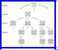
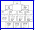
Consider a game such as chess, checkers, or tic-tac-toe, where there are two players. The players alternate moves, and the state of the game can be represented by a board position. Let us assume that there are a finite number of board positions and that the game has some sort of stopping rule to ensure termination. With each such game, we can associate a tree called the game tree. Each node of the tree represents a board position. With the root we associate the starting position. If board position x is associated with node n, then the children of n correspond to the set of allowable moves from board position x, and with each child is associated the resulting board position. For example, Fig. 10.16 shows part of the tree for tic-tac-toe.

Fig. 10.16. Part of the tic-tac-toe game tree.

The leaves of the tree correspond to board positions where there is no move, either because one of the players has won or because all squares are filled and a draw resulted. We associate a value with each node of the tree.

First we assign values to the leaves. Say the game is tic-tac-toe. Then a leaf is assigned -l, 0 or 1 depending on whether the board position corresponds to a loss, draw or win for player 1 (playing X).

http://www.ourstillwaters.org/stillwaters/csteaching/DataStructuresAndAlgorithms/mf1210.htm (19 of 40) [1.7.2001 19:27:46]

Data Structures and Algorithms: CHAPTER 10: Algorithm Design Techniques

The values are propagated up the tree according to the following rule. If a node corresponds to a board position where it is player 1's move, then the value is the maximum of the values of the children of that node. That is, we assume player 1 will make the move most favorable to himself i.e., that which produces the highest-valued outcome. If the node corresponds to player 2's move, then the value is the minimum of the values of the children. That is, we assume player 2 will make his most favorable move, producing a loss for player 1 if possible, and a draw as next preference.

Example 10.6. The values of the boards have been marked in Fig. 10.16. The leaves that are wins for O get value -1, while those that are draws get 0, and wins for X get + 1. Then we proceed up the tree. On level 8, where only one empty square remains, and it is X's move, the values for the unresolved boards is the "maximum" of the one child at level 9.

On level 7, where it is O's move and there are two choices, we take as a value for an interior node the minimum of the values of its children. The leftmost board shown on level 7 is a leaf and has value 1, because it is a win for X. The second board on level 7 has value min(0, -1) = -1, while the third board has value min(0, l) = 0. The one board shown at level 6, it being X's move on that level, has value max(l, -1, 0) = 1, meaning that there is some choice X can make that will win; in this case the win is immediate.

Note that if the root has value 1, then player 1 has a winning strategy. Whenever it is his turn he is guaranteed that he can select a move that leads to a board position of value 1. Whenever it is player 2's move he has no real choice but to select a moving leading to a board position of value 1, a loss for him. The fact that a game is assumed to terminate guarantees an eventual win for the first player. If the root has value 0, as it does in tic-tac-toe, then neither player has a winning strategy but can only guarantee himself a draw by playing as well as possible. If the root has value -1, then player 2 has a winning strategy.

Payoff Functions

The idea of a game tree, where nodes have values -1, 0, and l, can be generalized to trees where leaves are given any number (called the payoff) as a value, and the same rules for evaluating interior nodes applies: take the maximum of the children on those levels where player 1 is to move, and the minimum of the children on levels where player 2 moves.

As an example where general payoffs are useful, consider a complex game, like

http://www.ourstillwaters.org/stillwaters/csteaching/DataStructuresAndAlgorithms/mf1210.htm (20 of 40) [1.7.2001 19:27:46]

Data Structures and Algorithms: CHAPTER 10: Algorithm Design Techniques

chess, where the game tree, though finite, is so huge that evaluating it from the bottom up is not feasible. Chess programs work, in essence, by building for each board position from which it must move, the game tree with that board as root, extending downward for several levels; the exact number of levels depends on the speed with which the computer can work. As most of the leaves of the tree will be ambiguous, neither wins, losses, nor draws, each program uses a function of board positions that attempts to estimate the probability of the computer winning in that position. For example, the difference in material figures heavily into such an estimation, as do such factors as the defensive strength around the kings. By using this payoff function, the computer can estimate the probability of a win after making each of its possible next moves, on the assumption of subsequent best play by each side, and chose the move with the highest payoff.†

Implementing Backtrack Search

Suppose we are given the rules for a game,† that is, its legal moves and rules for termination. We wish to construct its game tree and evaluate the root. We could construct the tree in the obvious way, and then visit the nodes in postorder. The postorder traversal assures that we visit an interior node n after all its children, whereupon we can evaluate n by taking the min or max of the values of its children, as appropriate.

The space to store the tree can be prohibitively large, but by being careful we need never store more than one path, from the root to some node, at any one time. In Fig. 10.17 we see the sketch of a recursive program that represents the path in the tree by the sequence of active procedure calls at any time. That program assumes the following:

1.Payoffs are real numbers in a limited range, for example - 1 to + 1.

2.The constant ∞ is larger than any positive payoff and its negation is smaller than any negative payoff.

3.The type modetype is declared

type

modetype = (MIN, MAX)

4.There is a type boardtype declared in some manner suitable for the representation of board positions.

5.There is a function payoff that computes the payoff for any board that is a leaf (i.e., won, lost, or drawn position).

http://www.ourstillwaters.org/stillwaters/csteaching/DataStructuresAndAlgorithms/mf1210.htm (21 of 40) [1.7.2001 19:27:46]

Data Structures and Algorithms: CHAPTER 10: Algorithm Design Techniques

function search ( B: boardtype; mode: modetype ): real; { evaluates the payoff for board B, assuming it is

player 1's move if mode = MAX and player 2's move if mode = MIN. Returns the payoff }

var

C: boardtype; { a child of board B }

value: real; { temporary minimum or maximum value } begin

(1)if B is a leaf then

end; { search }

Fig. 10.17. Recursive backtrack search program.

Another implementation we might consider is to use a nonrecursive program that keeps a stack of boards corresponding to the sequence of active calls to search. The techniques discussed in Section 2.6 can be used to construct such a program.

Alpha-Beta Pruning

There is a simple observation that allows us to eliminate from consideration much of a typical game tree. In terms of Fig. 10.17, the for-loop of line (6) can skip over certain children, often many of the children. Suppose we have a node n, as in Fig. 10.18, and we have already determined that c1, the first of n's children, has a value of 20. As n is a max node, we know its value is at least 20. Now suppose that continuing with our search we find that d, a child of c2 has value 15. As c2, another child of n, is

http://www.ourstillwaters.org/stillwaters/csteaching/DataStructuresAndAlgorithms/mf1210.htm (22 of 40) [1.7.2001 19:27:46]

Data Structures and Algorithms: CHAPTER 10: Algorithm Design Techniques

a min node, we know the value of c2 cannot exceed 15. Thus, whatever value c2 has, it cannot affect the value of n or any parent of n.

It is thus possible in the situation of Fig. 10.18, to skip consideration of the children of c2 that we have not already examined. The general rules for

Fig. 10.18. Pruning the children of a node.

skipping or "pruning" nodes involves the notion of final and tentative values for nodes. The final value is what we have simply been calling the "value." A tentative value is an upper bound on the value of a min node, or a lower bound on the value of a max node. The rules for computing final and tentative values are the following.

1.If all the children of a node n have been considered or pruned, make the tentative value of n final.

2.If a max node n has tentative value v1 and a child with final value v2, then set the tentative value of n to max(v1, v2). If n is a min node, set its tentative value to min(v1, v2).

3.If p is a min node with parent q (a max node), and p and q have tentative values v1 and v2, respectively, with v1 ≤ v2, then we may prune all the

unconsidered children of p. We may also prune the unconsidered children of p if p is a max node (and therefore q is a min node) and v2 ≤ v1.

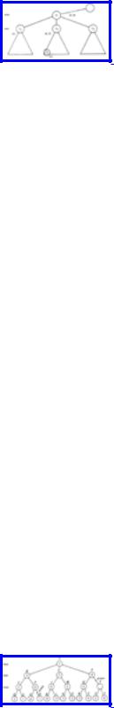
Example 10.7. Consider the tree in Fig. 10.19. Assuming values for the leaves as shown, we wish to calculate the value for the root. We begin a postorder traversal. After reaching node D, by rule (2) we assign a tentative value of 2, which is the final value of D, to node C. We then search E and return to C and then to B. By rule (1), the final value of C is fixed at 2 and the value of B is tentatively set to 2. The search continues down to G and then back to F. The value F is tentatively set to 6. By rule (3), with p and q equal to F and B, respectively, we may prune H. That is, there is no need to search node H, since the tentative value of F can never decrease and it is already greater than the value of B, which can never increase.

http://www.ourstillwaters.org/stillwaters/csteaching/DataStructuresAndAlgorithms/mf1210.htm (23 of 40) [1.7.2001 19:27:46]

Data Structures and Algorithms: CHAPTER 10: Algorithm Design Techniques

Fig. 10.19. A game tree.

Continuing our example, A is assigned a tentative value of 2 and the search proceeds to K. J is assigned a tentative value of 8. L does not determine the value of max node J. I is assigned a tentative value of 8. The search goes down to N, and M is assigned a tentative value of 5. Node O must be searched, since 5, the tentative value of M, is less than the tentative value of I. The tentative values of I and A are revised, and the search goes down to R. Eventually R and S are searched, and P is assigned a tentative value of 4. We need not search T or below, since that can only lower P's value and it is already too low to affect the value of A.

Branch-and-Bound Search

Games are not the only sorts of "problems" that can be solved exhaustively by searching a complete tree of possibilities. A wide variety of problems where we are asked to find a minimum or maximum configuration of some sort are amenable to solution by backtracking search over a tree of all possibilities. The nodes of the tree can be thought of as sets of configurations, and the children of a node n each represent a subset of the configurations that n represents. Finally, the leaves each represent single configurations, or solutions to the problem, and we may evaluate each such configuration to see if it is the best solution found so far.

If we are reasonably clever in how we design the search, the children of a node will each represent far fewer configurations than the node itself, so we need not go to too great a depth before reaching leaves. Lest this notion of searching appear too vague, let us take a concrete example.

Example 10.8. Recall from the previous section our discussion of the traveling salesman problem. There we gave a "greedy algorithm" for finding a good but not necessarily optimum tour. Now let us consider how we might find the optimum tour by systematically considering all tours. One way is to consider all permutations of the nodes, and evaluate the tour that visits the nodes in that order, remembering the best found so far. The time for such an approach is O(n!) on an n node graph, since we must consider (n--1)! different permutations,† and each permutation takes O(n) time to evaluate.

We shall consider a somewhat different approach that is no better than the above in the worst case, but on the average, when coupled with a technique called "branch- and-bound" that we shall discuss shortly, produces the answer far more rapidly than the "try all permutations" method. Start constructing a tree, with a root that represents all tours. Tours are what we called "configurations" in the prefatory material. Each

http://www.ourstillwaters.org/stillwaters/csteaching/DataStructuresAndAlgorithms/mf1210.htm (24 of 40) [1.7.2001 19:27:46]

Data Structures and Algorithms: CHAPTER 10: Algorithm Design Techniques

node has two children, and the tours that a node represents are divided by these children into two groups -- those that have a particular edge and those that do not. For example, Fig. 10.20 shows portions of the tree for the TSP instance from Fig. 10.15(a).

In Fig. 10.20 we have chosen to consider the edges in lexicographic order (a, b), (a, c), . . . ,(a, f), (b, c), . . . ,(b, f), (c, d), and so on. We could, of course pick any other order. Observe that not every node in the tree has two children. We can eliminate some children because the edges selected do not form part of a tour. Thus, there is no node for "tours containing (a, b), (a, c), and (a, d)," because a would have degree 3 and the result would not be a tour. Similarly, as we go down the tree we shall eliminate some nodes because some city would have degree less than 2. For example, we shall find no node for tours without (a, b), (a, c), (a, d), or (a, e).

Bounding Heuristics Needed for Branch- and-Bound

Using ideas similar to those in alpha-beta pruning, we can eliminate far more nodes of the search tree than would be suggested by Example 10.8. Suppose, to be specific, that our problem is to minimize some function, e.g., the cost of a tour in the TSP. Suppose also that we have a method for getting a lower bound on the cost of any solution among those in the set of solutions represented by some node n. If the best solution found so far costs less than the lower bound for node n, we need not explore any of the nodes below n.

Example 10.9. We shall discuss one way to get a lower bound on certain sets of solutions for the TSP, those sets represented by nodes in a tree of solutions as suggested in Fig. 10.20. First of all, suppose we wish a lower bound on all solutions to a given instance of the TSP. Observe that the cost of any tour can be expressed as one half the sum over all nodes n of the cost of the two tour edges adjacent to n. This remark leads to the following rule. The sum

Fig. 10.20. Beginning of a solution tree for a TSP instance.

of the two tour edges adjacent to node n is no less than the sum of the two edges of

http://www.ourstillwaters.org/stillwaters/csteaching/DataStructuresAndAlgorithms/mf1210.htm (25 of 40) [1.7.2001 19:27:46]