Data-Structures-And-Algorithms-Alfred-V-Aho

Data Structures and Algorithms: CHAPTER 10: Algorithm Design Techniques

least cost adjacent to n. Thus, no tour can cost less than one half the sum over all nodes n of the two lowest cost edges incident upon n.

For example, consider the TSP instance in Fig. 10.21. Unlike the instance in Fig. 10.15, the distance measure for edges is not Euclidean; that is, it bears no relation to the distance in the plane between the cities it connects. Such a cost measure might be traveling time or fare, for example. In this instance, the least cost edges adjacent to node a are (a, d), and (a, b), with a total cost of 5. For node b, we have (a, b) and (b, e), with a total cost of 6. Similarly, the two lowest cost edges adjacent to c, d, and e, total 8, 7, and 9, respectively. Our lower bound on the cost of a tour is thus (5+6+8+7+9)/2 = 17.5.

Fig. 10.21. An instance of TSP.

Now suppose we want a lower bound on the cost of a subset of tours defined by some node in the search tree. If the search tree is constructed as in Example 10.8, each node represents tours defined by a set of edges that must be in the tour and a set of edges that may not be in the tour. These constraints alter our choices for the two lowest-cost edges at each node. Obviously an edge constrained to be in any tour must be included among the two edges selected, no matter whether they are or are not lowest or second lowest in cost.† Similarly, an edge constrained to be out cannot be selected, even if its cost is lowest.

Thus, if we are constrained to include edge (a, e), and exclude (b, c), the two edges for node a are (a, d) and (a e), with a total cost of 9. For b we select (a b) and (b, e), as before, with a total cost of 6. For c, we cannot select (b, c), and so select (a, c) and (c, d), with a total cost of 9. For d we select (a, d) and (c, d), as before, while for e we must select (a, e), and choose to select (b, e). The lower bound for these constraints is thus (9+6+9+7+10)/2 = 20.5.

Now let us construct the search tree along the lines suggested in Example 10.8. We consider the edges in lexicographic order, as in that example. Each time we branch, by considering the two children of a node, we try to infer additional decisions regarding which edges must be included or excluded from tours represented by those nodes. The rules we use for these inference are:

1. If excluding an edge (x, y) would make it impossible for x or y to have as

http://www.ourstillwaters.org/stillwaters/csteaching/DataStructuresAndAlgorithms/mf1210.htm (26 of 40) [1.7.2001 19:27:46]

Data Structures and Algorithms: CHAPTER 10: Algorithm Design Techniques

many as two adjacent edges in the tour, then (x, y) must be included.

2.If including (x, y) would cause x or y to have more than two edges adjacent in the tour, or would complete a non-tour cycle with edges already included, then (x, y) must be excluded.

When we branch, after making what inferences we can, we compute lower bounds for both children. If the lower bound for a child is as high or higher than the lowest cost tour found so far, we can "prune" that child and need not construct or consider its descendants. Interestingly, there are situations where the lower bound for a node n is lower than the best solution so far, yet both children of n can be pruned because their lower bounds exceed the cost of the best solution so far.

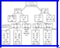
If neither child can be pruned, we shall, as a heuristic, consider the child with the smaller lower bound first, in the hope of more rapidly reaching a solution that is cheaper than the one so far found best.† After considering one child, we must consider again whether its sibling can be pruned, since a new best solution may have been found. For the instance of Fig. 10.21, we get the search tree of Fig. 10.22. To interpret nodes of that tree, it helps to understand that the capital letters are names of the search tree nodes. The numbers are the lower bounds, and we list the constraints applying to that node but none of its ancestors by writing xy if edge (x, y) must be

included and if (x, y) must be excluded. Also note that the constraints introduced at a node apply to all its descendants. Thus to get all the constraints applying at a node we must follow the path from that node to the root.

Lastly, let us remark that as for backtrack search in general, we construct the tree one node at a time, retaining only one path, as in the recursive algorithm of Fig. 10.17, or its nonrecursive counterpart. The nonrecursive version is probably to be preferred, so that we can maintain the list of constraints conveniently on a stack.

Example 10.10. Figure 10.22 shows the search tree for the TSP instance of Fig. 10.21. To see how it is constructed, we begin at the root A of Fig. 10.22. The first edge in lexicographic order is (a, b), so we consider the two children B and C,

corresponding to the constraints ab and , respectively. There is, as yet, no "best solution so far," so we shall consider both B and C eventually.‡ Forcing (a b) to be included does not raise the lower bound, but excluding it raises the bound to 18.5, since the two cheapest legal edges for nodes a and b now total 6 and 7, respectively, compared with 5 and 6 with no constraints. Following our heuristic, we shall consider the descendants of node B first.

The next edge in lexicographic order is (a, c). We thus introduce children D and E

http://www.ourstillwaters.org/stillwaters/csteaching/DataStructuresAndAlgorithms/mf1210.htm (27 of 40) [1.7.2001 19:27:46]

Data Structures and Algorithms: CHAPTER 10: Algorithm Design Techniques

corresponding to tours where (a, c) is included and excluded, respectively. In node D, we can infer that neither (a, d) nor (a, e) can be in a tour, else a would have too many edges incident. Following our heuristic we consider E before D, and branch on edge (a, d). The children F and G are introduced with lower bounds 18 and 23, respectively. For each of these children we know about three of the edges incident upon a, and so can infer something about the remaining edge (a, e).

Consider the children of F first. The first remaining edge in lexicographic order is (b, c). If we include (b, c), then, as we have included (a, b), we cannot include (b, d) or (b, e). As we have eliminated (a, e) and (b, e), we must have (c, e) and (d, e). We cannot have (c, d) or c and d would have three incident edges. We are left with one tour (a, b, c, e, d, a), whose cost is 23. Similarly, node I, where (b, c) is excluded, can be proved to represent only the tour (a b, e, c, d, a), of cost 21. That tour has the lowest cost found so far.

We now backtrack to E and consider its second child, G. But G has a lower bound of 23, which exceeds the best cost so far, 21. Thus we prune G. We now backtrack to B and consider its other child, D. The lower bound on D is 20.5, but since costs are integers, we know no tour represented by D can have cost less than 21. Since we already have a tour that cheap, we need not explore the descendants of D, and therefore prune D. Now we backtrack to A and consider its second child, C.

At the level of node C, we have only considered edge (a, b). Nodes J and K are introduced as children of C. J corresponds to those tours that have (a, c) but not (a, b), and its lower bound in 18.5. K corresponds to tours having neither (a, b) nor (a, c), and we may infer that those tours have (a, d) and (a, e). The lower bound for k is 21, and we may immediately prune k , since we already know a tour that is low in cost.

We next consider the children of J, which are L and M, and we prune M because its lower bound exceeds the best tour cost so far. The children of L are N and P, corresponding to tours that have (b, c), and that exclude (b, c). By considering the degree of nodes b and c, and remembering that the selected edges cannot form a cycle of fewer than all five cities, we can infer that nodes N and P each represent single tours. One of these, (a, c, b, e, d, a), has the lowest cost of any tour, 19. We have explored or pruned the entire tree and therefore end.

http://www.ourstillwaters.org/stillwaters/csteaching/DataStructuresAndAlgorithms/mf1210.htm (28 of 40) [1.7.2001 19:27:46]

Data Structures and Algorithms: CHAPTER 10: Algorithm Design Techniques

Fig. 10.22. Search tree for TSP solution.

10.5 Local Search Algorithms

Sometimes the following strategy will produce an optimal solution to a problem.

1.Start with a random solution.

2.Apply to the current solution a transformation from some given set of transformations to improve the solution. The improvement becomes the new "current" solution.

3.Repeat until no transformation in the set improves the current solution. The resulting solution may or may not be optimal. In principle, if the "given set of transformations" includes all the transformations that take one solution and replace it by any other, then we shall never stop until we reach an optimal solution. But then the time to apply (2) above is the same as the time needed to examine all solutions, and the whole approach is rather pointless.

The method makes sense when we can restrict our set of transformations to a small set, so we can consider all transformations in a short time; perhaps O(n2) or O(n3) transformations should be allowed when the problem is of "size" n. If the transformation set is small, it is natural to view the solutions that can be transformed to one another in one step as "close." The transformations are called "local transformations," and the method is called local search.

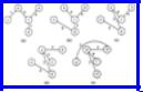
Example 10.11. One problem we can solve exactly by local search is the minimal spanning tree problem. The local transformations are those in which we take some edge not in the current spanning tree, add it to the tree, which must produce a unique cycle, and then eliminate exactly one edge of the cycle (presumably that of highest cost) to form a new tree.

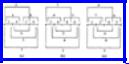
For example, consider the graph of Fig. 10.21. We might start with the tree shown in Fig. 10.23(a). One transformation we could perform is to add edge (d, e) and remove another edge in the cycle formed, which is (e, a, c, d, e). If we remove edge (a, e), we decrease the cost of the tree from 20 to 19. That transformation can be made, leaving the tree of Fig. 10.23(b), to which we again try to apply an improving transformation. One such is to insert edge (a, d) and delete edge (c, d) from the cycle formed. The result is shown in Fig. 10.23(c). Then we might introduce (a, b) and delete (b, c) as in Fig. 10.23(d), and subsequently introduce (b, e) in favor of (d, e). The resulting tree of Fig. 10.23(e) is minimal. We can check that every edge not in that tree has the

http://www.ourstillwaters.org/stillwaters/csteaching/DataStructuresAndAlgorithms/mf1210.htm (29 of 40) [1.7.2001 19:27:46]

Data Structures and Algorithms: CHAPTER 10: Algorithm Design Techniques

highest cost of any edge in the cycle it forms. Thus no transformation is applicable to Fig. 10.23(e).

The time taken by the algorithm of Example 10.11 on a graph of n nodes and e edges depends on the number of times we need to improve the solution. Just testing that no transformation is applicable could take O(ne) time, since e edges must be tried, and each could form a cycle of length nearly n Thus the algorithm is not as good as Prim's or Kruskal's algorithms, but serves as an example where an optimal solution can be obtained by local search.

Local Search Approximation Algorithms

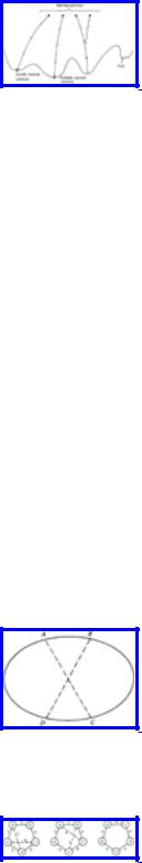
Local search algorithms have had their greatest effectiveness as heuristics for the solution to problems whose exact solutions require exponential time. A common method of search is to start with a number of random solutions, and apply the local transformations to each, until reaching a locally optimal solution, one that no transformation can improve. We shall frequently reach different locally optimal solutions, from most or all of the random starting solutions, as suggested in Fig. 10.24. If we are lucky, one of them will be

Fig. 10.23. Local search for a minimal spanning tree.

globally optimal, that is, as good as any solution.

In practice, we may not find a globally optimal solution as suggested in Fig. 10.24, since the number of locally optimal solutions may be enormous. However, we may at least choose that locally optimal solution that has the least cost among all those found. As the number of kinds of local transformations that have been used to solve various problems is great, we shall close the section with two examples -- the TSP, and a simple problem of "package placement."

The Traveling Salesman Problem

The TSP is one for which local search techniques have been remarkably successful. The simplest transformation that has been used is called "2-opting." It consists of taking any two edges, such as (A, B) and (C, D) in Fig. 10.25, removing them, and

http://www.ourstillwaters.org/stillwaters/csteaching/DataStructuresAndAlgorithms/mf1210.htm (30 of 40) [1.7.2001 19:27:46]

Data Structures and Algorithms: CHAPTER 10: Algorithm Design Techniques

reconnecting their endpoints to form a new tour. In Fig. 10.25, the new tour runs from B, clockwise to C, then along the edge (C, A), counterclockwise from A to D, and finally along the edge (D, B). If the sum of the lengths of (A, C) and (B, D) is less than the sum of the lengths of (A B) and (C, D), then we have an improved tour.† Note that we cannot

Fig. 10.24. Local search in the space of solutions.

connect A to D and B to C, as the result would not be a tour, but two disjoint cycles.

To find a locally optimal tour, we start with a random tour, and consider all pairs of nonadjacent edges, such as (A, B) and (C, D) in Fig. 10.25. If the tour can be improved by replacing these edges with (A, C) and (B, D), do so, and continue considering pairs of edges that have not been considered before. Note that the introduced edges (A, C) and (B, D) must each be paired with all the other edges of the tour, as additional improvements could result.

Example 10.12. Reconsider Fig. 10.21, and suppose we start with the tour of Fig. 10.26(a). We might replace (a, e) and (c, d), with a total cost of 12, by (a, d) and (c, e), with a total cost of 10, as shown in Fig. 10.26(b). Then we might replace (a, b) and (c, e) by (a, c) and (b, e), giving the optimal tour shown in Fig. 10.26(c). One can check that no pair of edges can be removed from Fig. 10.26(c) and be profitably replaced by crossing edges with the same endpoints. As one case in point, (b, c) and (d, e) together have the relatively high cost of 10. But (c, e) and (b, d) are worse, costing 14 together.

Fig. 10.25. 2-opting.

http://www.ourstillwaters.org/stillwaters/csteaching/DataStructuresAndAlgorithms/mf1210.htm (31 of 40) [1.7.2001 19:27:46]

Data Structures and Algorithms: CHAPTER 10: Algorithm Design Techniques

Fig. 10.26. Optimizing a TSP instance by 2-opting.

We can generalize 2-opting to k-opting for any constant k , where we remove up to k edges and reconnect the remaining pieces in any order so that result is a tour. Note that we do not require the removed edges to be nonadjacent in general, although for the 2-opting case there was no point in considering the removal of two adjacent edges. Also note that for k >2, there is more than one way to connect the pieces. For example, Fig. 10.27 shows the general process of 3-opting using any of the following eight sets of edges.

Fig. 10.27. Pieces of a tour after removing three edges.

It is easy to check that, for fixed k , the number of different k-opting transformations we need to consider if there are n vertices is O(n k). For example, the exact number is n(n-3)/2 for k = 2. The time taken to obtain a locally optimal tour may be considerably higher than this, however, since we could make many local transformations before reaching a locally optimum tour, and each improving transformation introduces new edges that may participate in later transformations that improve the tour still further. Lin and Kernighan [1973] have found that variable- depth-opting is in practice a very powerful method and has a good chance of getting the optimum tour on 40-100 city problems.

Package Placement

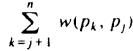
The one-dimensional package placement problem can be stated as follows. We have an undirected graph, whose vertices we call "packages." The edges are labeled by "weights," and the weight w(a, b) of edge (a, b) is the number of "wires" between packages a and b. The problem is to order the vertices p1, p2,..., pn, such that the sum of [i-j] w(pi, pj) over all pairs i and j is minimized. That is, we want to minimize the sum of the lengths of the wires needed to connect all the packages with the required number of wires.

The package placement problem has had a number of applications. For example, the "packages" could be logic cards on a rack, and the weight of an interconnection between cards is the number of wires connecting them. A similar problem comes up when we try to design integrated circuits from arrays of standard modules and

http://www.ourstillwaters.org/stillwaters/csteaching/DataStructuresAndAlgorithms/mf1210.htm (32 of 40) [1.7.2001 19:27:46]

Data Structures and Algorithms: CHAPTER 10: Algorithm Design Techniques

interconnections between them. A generalization of the one-dimensional package placement problem allows placement of "packages," which have height and width, in a two-dimensional region, while minimizing the sum of the lengths of the wires between packages. This problem also has application to the design of integrated circuits, among other areas.

There are a number of local transformations we could use to find local optima for instances of the one-dimensional package placement problem. Here are several.

1.Interchange adjacent packages pi and pi+1 if the resulting order is less costly.

Let L(j) be the sum of the weights of the edges extending to the left of pj, i.e.,

. Similarly, let R(j) be . Improvement results if L(i) - R(i) + R(i+ 1) - L(i+ 1) + 2w(pi, pi+1) is negative. The reader should verify this formula by computing the costs before and after the interchange and taking the difference.

2.Take a package pi and insert it between pj and pj+1 for some i and j.

3.Interchange any two packages pi and pj.

Example 10.13. Suppose we take the graph of Fig. 10.21 to represent a package placement instance. We shall restrict ourselves to the simple transformation set (1). An initial placement, a, b, c, d, e, is shown in Fig. 10.28(a); it has a cost of 97. Note that the cost function weights edges by their distance, so (a, e) contributes 4x7 = 28 to the cost of 97. Let us consider interchanging d with e. We have L(d) = 13, R(d) = 6, L(e) = 24, and R(e) = 0. Thus L(d)-R(d)+R(e)- L(e)+2w(d, e) = -5, and we can interchange d and e to improve the placement to (a, b, c, e, d), with a cost of 92 as shown in Fig. 10.28(b).

In Fig. 10.28(b), we can interchange c with e profitably, producing Fig. 10.28(c), whose placement (a, b, e, c, d) has a cost of 91. Fig. 10.28(c) is locally optimal for set of transformations (1). It is not globally optimal; (a, c, e, d, b) has a cost of 84.

As with the TSP, we cannot estimate closely the time it takes to reach a local optimum. We can only observe that for set of transformations (1), there are only n-1 transformations to consider. Further, if we compute L(i) and R(i) once, we only have to change them when pi is interchanged with pi-1 or pi+1. Moreover, the recalculation is easy. If pi and pi+1 are interchanged, for example, then the new L(i) and R(i) are,

respectively, L(i+1) - w(pi, pi+1) and R(i+1) + w(pi, pi+1). Thus O(n) time suffices to test for an improving transformation and to recalculate the L(i)'s and R(i)'s. We also need only O(n) time to initialize the L(i)'s and R(i)'s, if we use the recurrence

http://www.ourstillwaters.org/stillwaters/csteaching/DataStructuresAndAlgorithms/mf1210.htm (33 of 40) [1.7.2001 19:27:46]

Data Structures and Algorithms: CHAPTER 10: Algorithm Design Techniques

Fig. 10.28. Local optimizations.

L(1) = 0

L(i) = L(i-1) + w(pi-1, pi)

and a similar recurrence for R.

In comparison, the sets of transformations (2) and (3) each have O(n2) members. It will therefore take O(n2) time just to confirm that we have a locally optimal solution. However, as for set (1), we cannot closely bound the total time taken when a sequence of improvements are made, since each improvement can create additional opportunities for improvement.

Exercises

10.1

How many moves do the algorithms for moving n disks in the Towers of Hanoi problem take?

Prove that the recursive (divide and conquer) algorithm for the Tower *10.2 of Hanoi and the simple nonrecursive algorithm described at the

beginning of Section 10.1 perform the same steps.

10.3

Show the actions of the divide-and-conquer integer multiplication algorithm of Fig. 10.3 when multiplying 1011 by 1101.

Generalize the tennis tournament construction of Section 10.1 to tournaments where the number of players is not a power of two. Hint. If the number of players n is odd, then one player must receive a bye

*10.4 (not play) on any given day, and it will take n days, rather than n-1 to complete the tournament. However, if there are two groups with an odd number of players, then the players receiving the bye from each group may actually play each other.

http://www.ourstillwaters.org/stillwaters/csteaching/DataStructuresAndAlgorithms/mf1210.htm (34 of 40) [1.7.2001 19:27:46]

Data Structures and Algorithms: CHAPTER 10: Algorithm Design Techniques

We can recursively define the number of combinations of m things out of n, denoted , for n ³1 and 0 £ m £ n, by

a. Give a recursive function to compute

10.5

b.What is its worst-case running time as a function of n?

c.Give a dynamic programming algorithm to compute .Hint. The algorithm constructs a

table generally known as Pascal's triangle.

d.What is the running time of your answer to (c) as a function of n.

One way to compute the number of combinations of m things out of n is to calculate (n)(n-1)(n-2) × × × (n-m+l)/(1)(2) × × × (m).

a. What is the worst case running time of this algorithm as a

http://www.ourstillwaters.org/stillwaters/csteaching/DataStructuresAndAlgorithms/mf1210.htm (35 of 40) [1.7.2001 19:27:46]