Data-Structures-And-Algorithms-Alfred-V-Aho

Data Structures and Algorithms: CHAPTER 10: Algorithm Design Techniques

emerged is that it is generally advantageous to balance competing costs wherever possible. For example in Chapter 5 we saw that the 2-3 tree balanced the costs of searching with those of inserting, while more straightforward methods take O(n) steps either for each lookup or for each insertion, even though the other operation can be done in a constant number of steps.

Similarly, for divide-and-conquer algorithms, we are generally better off if the subproblems are of approximately equal size. For example, insertion sort can be viewed as partitioning a problem into two subproblems, one of size 1 and one of size n - 1, with a maximum cost of n steps to merge. This gives a recurrence

T(n) = T(1) + T(n - 1) + n

which has an O(n2) solution. Mergesort, on the other hand, partitions the problems into two subproblems each of size n/2 and has O(nlogn) performance. As a general principle, we often find that partitioning a problem into

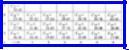
Fig. 10.4. A round-robin tournament for eight players.

equal or nearly equal subproblems is a crucial factor in obtaining good performance.

10.2 Dynamic Programming

Often there is no way to divide a problem into a small number of subproblems whose solution can be combined to solve the original problem. In such cases we may attempt to divide the problem into as many subproblems as necessary, divide each subproblem into smaller subproblems and so on. If this is all we do, we shall likely wind up with an exponential-time algorithm.

Frequently, however, there are only a polynomial number of subproblems, and thus we must be solving some subproblem many times. If instead we keep track of the solution to each subproblem solved, and simply look up the answer when needed, we would obtain a polynomial-time algorithm.

It is sometimes simpler from an implementation point of view to create a table of the solutions to all the subproblems we might ever have to solve. We fill in the table

http://www.ourstillwaters.org/stillwaters/csteaching/DataStructuresAndAlgorithms/mf1210.htm (6 of 40) [1.7.2001 19:27:46]

Data Structures and Algorithms: CHAPTER 10: Algorithm Design Techniques

without regard to whether or not a particular subproblem is actually needed in the overall solution. The filling-in of a table of subproblems to get a solution to a given problem has been termed dynamic programming, a name that comes from control theory.

The form of a dynamic programming algorithm may vary, but there is the common theme of a table to fill and an order in which the entries are to be filled. We shall illustrate the techniques by two examples, calculating odds on a match like the World Series, and the "triangulation problem."

World Series Odds

Suppose two teams, A and B, are playing a match to see who is the first to win n games for some particular n. The World Series is such a match, with n = 4. We may suppose that A and B are equally competent, so each has a 50% chance of winning any particular game. Let P(i, j) be the probability that if A needs i games to win, and B needs j games, that A will eventually win the match. For example, in the World Series, if the Dodgers have won two games and the Yankees one, then i = 2, j = 3, and P(2, 3), we shall discover, is 11/16.

To compute P(i, j), we can use a recurrence equation in two variables. First, if i = 0 and j > 0, then team A has won the match already, so P(0, j) = 1. Similarly, P(i, 0) = 0 for i > 0. If i and j are both greater than 0, at least one more game must be played, and the two teams each win half the time. Thus, P(i, j) must be the average of P(i - 1, j) and P(i, j - 1), the first of these being the probability A will win the match if it wins the next game and the second being the probability A wins the match even though it loses the next game. To summarize:

P(i, j) = 1 if i = 0 and j > 0 = 0 if i > 0 and j = 0

= (P(i - 1, j) + P(i, j - 1))/2 if i > 0 and j > 0 (10.4)

If we use (10.4) recursively as a function, we can show that P(i, j) takes no more than time O(2i+j). Let T(n) be the maximum time taken by a call to P(i, j), where i + j = n. Then from (10.4),

T(1) = c

T(n) = 2T(n - 1) + d

http://www.ourstillwaters.org/stillwaters/csteaching/DataStructuresAndAlgorithms/mf1210.htm (7 of 40) [1.7.2001 19:27:46]

Data Structures and Algorithms: CHAPTER 10: Algorithm Design Techniques

for some constants c and d. The reader may check by the means discussed in the previous chapter that T(n) ≤ 2n- 1c + (2n-1-1)d, which is O(2n) or O(2i+j).

We have thus proven an exponential upper bound on the time taken by the recursive computation of P(i, j). However, to convince ourselves that the recursive formula for P(i, j) is a bad way to compute it, we need to get a big-omega lower bound. We leave it as an exercise to show that when we call P(i, j), the total number

of calls to P that gets made is , the number of ways to choose i things out of i+j. If i = j, that number is , where n = i+j. Thus, T(n) is , and

in fact, we can show it is also. While grows asymptotically more slowly than 2n, the difference is not great, and T(n) grows far too fast for the recursive calculation of P(i, j) to be practical.

The problem with the recursive calculation is that we wind up computing the same P(i, j) repeatedly. For example, if we want to compute P(2, 3), we compute, by (10.4), P(1, 3) and P(2, 2). P(1, 3) and P(2, 2) both require the computation of P(1, 2), so we compute that value twice.

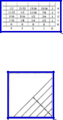
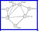
A better way to compute P(i, j) is to fill in the table suggested by Fig. 10.5. The bottom row is all 0's and the rightmost column all 1's by the first two lines of (10.4). By the last line of (10.4), each other entry is the average of the entry below it and the entry to the right. Thus, an appropriate way to fill in the table is to proceed in diagonals beginning at the lower right corner, and proceeding up and to the left along diagonals representing entries with a constant value of i+j, as suggested in Fig. 10.6. This program is given in Fig. 10.7, assuming it works on a two-dimensional array P of suitable size.

Fig. 10.5. Table of odds.

Fig. 10.6. Pattern of computation.

http://www.ourstillwaters.org/stillwaters/csteaching/DataStructuresAndAlgorithms/mf1210.htm (8 of 40) [1.7.2001 19:27:46]

Data Structures and Algorithms: CHAPTER 10: Algorithm Design Techniques

The analysis of function odds is easy. The loop of lines (4)-(5) takes O(s) time, and that dominates the O(1) time for lines (2)-(3). Thus, the outer loop takes time

, where i+j = n. Thus dynamic

Fig. 10.7. Odds calculation.

programming takes O(n2) time, compared with for the straightforward

approach. Since grows wildly faster than n2, we would prefer dynamic programming to the recursive approach under essentially any circumstances.

The Triangulation Problem

As another example of dynamic programming, consider the problem of triangulating a polygon. We are given the vertices of a polygon and a distance measure between each pair of vertices. The distance may be the ordinary (Euclidean) distance in the plane, or it may be an arbitrary cost function given by a table. The problem is to select a set of chords (lines between nonadjacent vertices) such that no two chords cross each other, and the entire polygon is divided into triangles. The total length (distance between endpoints) of the chords selected must be a minimum. We call such a set of chords a minimal triangulation.

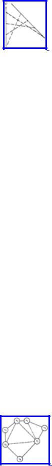
Example 10.1. Figure 10.8 shows a seven-sided polygon and the (x, y) coordinates of its vertices. The distance function is the ordinary Euclidean distance. A triangulation,

http://www.ourstillwaters.org/stillwaters/csteaching/DataStructuresAndAlgorithms/mf1210.htm (9 of 40) [1.7.2001 19:27:46]

Data Structures and Algorithms: CHAPTER 10: Algorithm Design Techniques

which happens not to be minimal, is shown by dashed lines. Its cost is the sum of the lengths of the chords (v0, v2), (v0, v3), (v0, v5), and (v3, v5), or

.

As well as being interesting in its own right, the triangulation problem has a number of useful applications. For example, Fuchs, Kedem, and Uselton [1977] used a generalization of the triangulation problem for the following purpose. Consider the problem of shading a two-dimensional picture of an object whose surface is defined by a collection of points in 3-space. The light source comes from a given direction, and the brightness of a point on the surface depends on the angles between the direction of light, the direction of the viewer's eye, and a perpendicular to the surface at that point. To estimate the direction of the surface at a point, we can compute a minimum triangulation

Fig. 10.8. A heptagon and a triangulation.

of the points defining the surface.

Each triangle defines a plane in a 3-space, and since a minimum triangulation was found, the triangles are expected to be very small. It is easy to find the direction of a perpendicular to a plane, so we can compute the light intensity for the points of each triangle, on the assumption that the surface can be treated as a triangular plane in a given region. If the triangles are not sufficiently small to make the light intensity look smooth, then local averaging can improve the picture.

Before proceeding with the dynamic programming solution to the triangulation problem, let us state two observations about triangulations that will help us design the algorithm. Throughout we assume we have a polygon with n vertices v0, v1, . . . , vn-1, in clockwise order.

Fact 1. In any triangulation of a polygon with more than three vertices, every pair of adjacent vertices is touched by at least one chord. To see this, suppose neither vi nor vi+1† were touched by a chord. Then the region that edge (vi, vi+1) bounds would have to include edges (vi-1, vi), (vi+1, Vi+2) and at least one additional edge. This region then would not be a triangle.

http://www.ourstillwaters.org/stillwaters/csteaching/DataStructuresAndAlgorithms/mf1210.htm (10 of 40) [1.7.2001 19:27:46]

Data Structures and Algorithms: CHAPTER 10: Algorithm Design Techniques

Fact 2. If (vi, vj) is a chord in a triangulation, then there must be some vk such that (vi, vk) and (vk, vj) are each either edges of the polygon or chords. Otherwise, (vi, vj) would bound a region that was not a triangle.

To begin searching for a minimum triangulation, we pick two adjacent vertices, say v0 and v1. By the two facts we know that in any triangulation, and therefore in the minimum triangulation, there must be a vertex vk such that (v1, vk) and (vk, v0) are chords or edges in the triangulation. We must therefore consider how good a triangulation we can find after selecting each possible value for k. If the polygon has n vertices, there are a total of (n-2) choices to make.

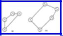
Each choice of k leads to at most two subproblems, which we define to be polygons formed by one chord and the edges in the original polygon from one end of the chord to the other. For example, Fig. 10.9 shows the two subproblems that result if we select the vertex v3.

Fig. 10.9. The two subproblems after selecting v3.

Next, we must find minimum triangulations for the polygons of Fig. 10.9(a) and

(b). Our first instinct is that we must again consider all chords emanating from two adjacent vertices. For example, in solving Fig. 10.9(b), we might consider choosing chord (v3, v5), which leaves subproblem (v0, v3, v5, v6), a polygon two of whose sides, (v0, v3) and (v3, v5), are chords of the original polygon. This approach leads to an exponential-time algorithm.

However, by considering the triangle that involves the chord (v0, vk) we never have to consider polygons more than one of whose sides are chords of the original polygon. Fact 2 tells us that, in the minimal triangulation, thechord in the subproblem, such as (v0, v3) in Fig. 10.9(b), must make a triangle with one of the other vertices. For example, if we select v4, we get the triangle (v0, v3, v4) and the subproblem (v0, v4, v5, v6) which has only one chord of the original polygon. If we try v5, we get the subproblems (v3, v4, v5) and (v0, v5, v6), with chords (v3, v5) and (v0, v5) only.

In general, define the subproblem of size s beginning at vertex vi, denoted Sis, to

http://www.ourstillwaters.org/stillwaters/csteaching/DataStructuresAndAlgorithms/mf1210.htm (11 of 40) [1.7.2001 19:27:46]

Data Structures and Algorithms: CHAPTER 10: Algorithm Design Techniques

be the minimal triangulation problem for the polygon formed by the s vertices beginning at vi and proceeding clockwise, that is, vi, vi+1, ..., vi+s-1. The chord in Sis is

(vi, vi+s-1). For example, Fig. 10.9(a) is S04 and Fig. 10.9(b) is S35. To solve Sis we must consider the following three options.

1.We may pick vertex vi+s-2 to make a triangle with the chords (vi, vi+s-1) and (vi, vi+s-2) and third side (vi+s-2, vi+s-l), and then solve the subproblem Si,s-1.

2.We may pick vertex vi+1 to make a triangle with the chords (vi, vi+s-1) and (vi+1, vi+s-1) and third side (vi, vi+1), and then solve the subproblem Si + 1,s-1.

3.For some k between 2 and s-3 we may pick vertex vi+k and form a triangle with sides (vi, vi+k), (vi+k, vi+s-1), and (vi, vi+s-1) and then solve subproblems

Si,k+1 and Si+k,s-k.

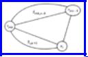
If we remember that "solving" any subproblem of size three or less requires no action, we can summarize (1)-(3) by saying that we pick some k between 1 and s-2 and solve subproblems Si,k+1 and Si+k,s-k. Figure 10.10 illustrates this division into subproblems.

Fig. 10.10. Division of Sis into subproblems.

If we use the obvious recursive algorithm implied by the above rules to solve subproblems of size four or more, then it is possible to show that each call on a subproblem of size s gives rise to a total of 3s-4 recursive calls, if we "solve" subproblems of size three or less directly and count only calls on subproblems of size four or more. Thus the number of subproblems to be solved is exponential in s. Since our initial problem is of size n, where n is the number of vertices in the given polygon, the total number of steps performed by this recursive procedure is exponential in n.

Yet something is clearly wrong in this analysis, because we know that besides the original problem, there are only n(n-4) different subproblems that ever need to be solved. They are represented by Sis, where 0 ≤ i < n and 4 ≤ s < n. Evidently not all the subproblems solved by the recursive procedure are different. For example, if in Fig. 10.8 we choose chord (v0, v3), and then in the subproblem of Fig. 10.9(b) we pick v4, we have to solve subproblem S44. But we would also have to solve this

http://www.ourstillwaters.org/stillwaters/csteaching/DataStructuresAndAlgorithms/mf1210.htm (12 of 40) [1.7.2001 19:27:46]

Data Structures and Algorithms: CHAPTER 10: Algorithm Design Techniques

problem if we first picked chord (v0, v4), or if we picked (v1, v4) and then, when solving subproblem S45, picked vertex v0 to complete a triangle with v1 and v4.

This suggests an efficient way to solve the triangulation problem. We make a table giving the cost Cis of triangulating Sis for all i and s. Since the solution to any given problem depends only on the solution to problems of smaller size, the logical order in which to fill in the table is in size order. That is, for sizes s = 4, 5, . . . ,n-1 we fill in the minimum cost for problems Sis, for all vertices i. It is convenient to include problems of size 0 £ s < 4 as well, but remember that Sis has cost 0 if s < 4.

By rules (1)-(3) above for finding subproblems, the formula for computing Cis for s ³ 4 is:

where D(vp, vq) is the length of the chord between vertices vp and vq, if vp and vq are not adjacent points on the polygon; D(vp, vq) is 0 if vp and vq are adjacent.

Example 10.2. Figure 10.11 holds the table of costs for Si,s for 0 £ i £ 6 and 4 £ s £

6, based on the polygon and distances of Fig. 10.8. The costs for the rows with s < 3 are all zero. We have filled in the entry C07, in column 0 and the row for s = 7. This entry, like all in that row, represents the triangulation of the entire polygon. To see that, just notice that we can, if we wish, consider the edge (v0, v6) to be a chord of a larger polygon and the polygon of Fig. 10.8 to be a subproblem of this polygon, which has a series of additional vertices extending clockwise from v6 to v0. Note that the entire row for s = 7 has the same value as C07, to within the accuracy of the computation.

Let us, as an example, show how the entry 38.09 in the column for i = 6 and row for s = 5 is filled in. According to (10.5) the value of this entry, C65, is the minimum of three sums, corresponding to k = 1, 2, or 3. These sums are:

C62 + C04 + D

(v6, v0) + D(v0, v3)

C63 + C13 + D

http://www.ourstillwaters.org/stillwaters/csteaching/DataStructuresAndAlgorithms/mf1210.htm (13 of 40) [1.7.2001 19:27:46]

Data Structures and Algorithms: CHAPTER 10: Algorithm Design Techniques

(v6, v1) + D(v1, v3)

C64 + C22 + D

(v6, v2) + D(v2, v3)

Fig. 10.11 Table of Cis's.

The distances we need are calculated from the coordinates of the vertices as:

D(v2, v3) =

D(v6, v0) = 0

(since these are polygon edges, not chords, and are present "for free")

D(v6, v2) = 26.08

D(v1, v3) = 16.16

D(v6, v1) = 22.36

D(v0, v3) = 21.93

The three sums above are 38.09, 38.52, and 43.97, respectively. We may conclude that the minimum cost of the subproblem S65 is 38.09. Moreover, since the first sum was smallest, we know that to achieve this minimum we must utilize the subproblems S62 and S04, that is, select chord (v0, v3) and then solve S64 as best we can; chord (v1, v3) is the preferred choice for that subproblem.

There is a useful trick for filling out the table of Fig. 10.11 according to the formula (10.5). Each term of the min operation in (10.5) requires a pair of entries. The first pair, for k = 1, can be found in the table (a) at the "bottom" (the row for s = 2)† of the column of the element being computed, and (b) just below and to the right‡ of the element being computed. The second pair is (a) next to the bottom of the column, and (b) two positions down and to the right. Fig. 10.12 shows the two lines of entries we follow to get all the pairs of entries we need to consider simultaneously. The pattern -- up the column and down the diagonal -- is a common one in filling

http://www.ourstillwaters.org/stillwaters/csteaching/DataStructuresAndAlgorithms/mf1210.htm (14 of 40) [1.7.2001 19:27:46]

Data Structures and Algorithms: CHAPTER 10: Algorithm Design Techniques

tables during dynamic programming.

Fig. 10.12. Pattern of table scan to compute one element.

Finding Solutions from the Table

While Fig. 10.11 gives us the cost of the minimum triangulation, it does not immediately give us the triangulation itself. What we need, for each entry, is the value of k that produced the minimum in (10.5). Then we can deduce that the solution consists of chords (vi, vi+k), and (vi+k, vi+s-1) (unless one of them is not a chord, because k = 1 or k = s-2), plus whatever chords are implied by the solutions to Si,k+1 and Si+k,s-k. It is useful, when we compute an element of the table, to include with it the value of k that gave the best solution.

Example 10.3. In Fig. 10.11, the entry C07, which represents the solution to the entire problem of Fig. 10.8, comes from the terms for k = 5 in (10.5). That is, the problem S07 is split into S06 and S52; the former is the problem with six vertices v0, v1, . . . ,v5, and the latter is a trivial "problem" of cost 0. Thus we introduce the chord (v0, v5) of cost 22.09 and must solve S06.

The minimum cost for C06 comes from the terms for k = 2 in (10.5), whereby the problem S06 is split into S03 and S24. The former is the triangle with vertices v0, v1, and v2, while the latter is the quadrilateral defined by v2, v3, v4, and v5. S03 need not be solved, but S24 must be, and we must include the costs of chords (v0, v2) and (v2, v5) which are 17.89 and 19.80, respectively. We find the minimum value for C24 is assumed when k = 1 in (10.5), giving us the subproblems C22 and C33, both of which have size less than or equal to three and therefore cost 0. The chord (v3, v5) is introduced, with a cost of 15.65.

http://www.ourstillwaters.org/stillwaters/csteaching/DataStructuresAndAlgorithms/mf1210.htm (15 of 40) [1.7.2001 19:27:46]