Data-Structures-And-Algorithms-Alfred-V-Aho

Data Structures and Algorithms: CHAPTER 8: Sorting

(1)for i := l to n do

{push A[i] onto the front of the bin for its key }

(3)for v := succ(lowkey) to highkey do

{concatenate all the bins onto the end of B[lowkey] }

(4) CONCATENATE (B[lowkey], B[v])

end; { binsort }

Fig. 8.20. The abstract binsort program.

Analysis of Binsort

We claim that if there are n elements to be sorted, and there are m different key values (hence m different bins), then the program of Fig. 8.20 takes O(n + m) time, if the proper data structure for bins is used. In particular, if m ≤ n, then binsort takes O(n) time. The data structure we have in mind is a linked list. Pointers to list ends, as indicated in Fig. 8.19, are useful but not required.

The loop of lines (1 - 2) of Fig. 8.20, which places the records in bins, takes O(n) time, since the INSERT operation of line (2) requires constant time, the insertion always occurring at the beginning of the list. For the loop of lines (3 - 4), concatenating the bins, temporarily assume that pointers to the ends of lists exist. Then step (4) takes constant time, so the loop takes O(m) time. Hence the entire binsort program takes O(n + m) time.

If pointers to the ends of lists do not exist, then in line (4) we must spend time running down to the end of B[v] before concatenating it to B[lowkey]. In this manner, the end of B[lowkey] will always be available for the next concatenation. The extra time spent running to the end of each bin once totals O(n), since the sum of the lengths of the bins is n. This extra time does not affect the order of magnitude of running time for the algorithm, since O(n) is no greater than O(n + m).

Sorting Large Key Sets

If m, the number of keys, is no greater than n, the number of elements, then the O(n + m) running time of Fig. 8.20 is really O(n). But what if m=n2, say. Evidently Fig. 8.20 will take O(n + n2), which is O(n2) time. But can we still take advantage of the fact that the key set is limited and do better? The surprising answer is that even if the set of possible key values is 1,2 , . . . , nk, for any fixed k, then there is a

http://www.ourstillwaters.org/stillwaters/csteaching/DataStructuresAndAlgorithms/mf1208.htm (26 of 44) [1.7.2001 19:22:21]

Data Structures and Algorithms: CHAPTER 8: Sorting

generalization of the binsorting technique that takes only O(n) time.

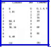
Example 8.6. Consider the specific problem of sorting n integers in the range 0 to n2 - 1. We sort the n integers in two phases. The first phase appears not to be of much help at all, but it is essential. We use n bins, one for each of the integers 0, 1 , . . . , n - 1. We place each integer i on the list to be sorted, into the bin numbered i mod n. However, unlike Fig. 8.20, it is important that we append each integer to the end of the list for the bin, not the beginning. If we are to append efficiently, we require the linked list representation of bins, with pointers to list ends.

For example, suppose n = 10, and the list to be sorted is the perfect squares from 02 to 92 in the random order 36, 9, 0, 25, 1, 49, 64, 16, 81, 4. In this case, where n = 10, the bin for integer i is just the rightmost digit of i written in decimal. Fig. 8.21(a) shows the placement of our list into bins. Notice that integers appear in bins in the same order that they appear in the original list; e.g., bin 6 has contents 36, 16, not 16, 36, since 36 precedes 16 on the original list.

Now, we concatenate the bins in order, producing the list

from Fig. 8.21(a). If we use the linked list data structure with pointers to list ends, then the placement of the n integers into bins and the concatenation of the bins can each be done in O(n) time.

The integers on the list created by concatenating the bins are redistributed into bins, but using a different bin selection strategy. Now place integer i into bin [i/n], that is, the greatest integer equal to or less than i/n. Again, append integers to the ends of the lists for the bins. When we now concatenate the bins in order, we find the list is sorted.

For our example, Fig. 8.21(b) shows the list (8.10) distributed into bins, with i going into bin [i/10].

To see why this algorithm works, we have only to notice that when several integers are placed in one bin, as 0, 1, 4, and 9 were placed in bin 0, they must be in increasing order, since the list (8.10) resulting from the first pass ordered them by rightmost digit. Hence, in any bin the rightmost digits must form an increasing sequence. Of course, any integer placed in bin i must precede an integer placed in a bin higher than i, so concatenating the bins in order produces the sorted list.

http://www.ourstillwaters.org/stillwaters/csteaching/DataStructuresAndAlgorithms/mf1208.htm (27 of 44) [1.7.2001 19:22:21]

Data Structures and Algorithms: CHAPTER 8: Sorting

More generally, we can think of the integers between 0 and n2 - 1 as

Fig. 8.21. Two-pass binsorting.

two-digit numbers in base n and use the same argument to see that the sorting strategy works. Consider the integers i = an + b and j = cn + d, where a, b, c, and d are each in the range 0 to n - l; i.e., they are base- n digits. Suppose i<j. Then, a>c is not possible, so we may assume a£c. If a<c, then i appears in a lower bin than j after the second pass, so i will precede j in the final order. If a=c, then b must be less than d. Then after the first pass, i precedes j, since i was placed in bin b and j in bin d. Thus, while both i and j are placed in bin a (the same as bin c), i is inserted first, and j must follow it in the bin.

General Radix Sorting

Suppose keytype is a sequence of fields, as in

type

keytype = record day: 1..31;

month: (jan , . . . , dec); (8.11) year: 1900..1999

end;

or an array of elements of the same type, as in

We shall assume from here that keytype consists of k components, f1,f2, . . . ,fk of types t1, t2, . . . , tk. For example, in (8.11) t1 = 1..31, t2 = (jan , . . . , dec), and t3 = 1900..1999. In (8.12), k = 10, and t1 = t2 = × × × = tk = char.

http://www.ourstillwaters.org/stillwaters/csteaching/DataStructuresAndAlgorithms/mf1208.htm (28 of 44) [1.7.2001 19:22:21]

Data Structures and Algorithms: CHAPTER 8: Sorting

Let us also assume that we desire to sort records in the lexicographic order of their keys. That is, key value (a1, a2, . . . ,ak) is less than key value (b1, b2, . . . ,bk), where ai and bi are the values in field fi, for i = 1, 2, . . . ,k, if either

1.a1 < b1, or

2.a1 = b1 and a2 < b2, or

.

.

.

k. a1 = b1, a2 = b2, . . . ,ak - 1=bk - 1, and ak < bk.

That is, for some j between 0 and k - 1, a1 = b1, . . . , aj = bj, † and aj + 1 <bj + 1.

We can view keys of the type defined above as if key values were integers expressed in some strange radix notation. For example, (8.12) where each field is a character, can be viewed as expressing integers in base 128, or however many characters there are in a character set for the machine at hand. Type definition (8.11) can be viewed as if the rightmost place were in base 100 (corresponding to the values between 1900 and 1999), the next place in base 12, and the third in base 31. Because of this view, generalized binsort has become known as radix sorting. In the extreme, we can even use it to sort integers up to any fixed limit by seeing them as arrays of digits in base 2, or another base.

The key idea behind radix sorting is to binsort all the records, first on fk, the "least significant digit," then concatenate the bins, lowest value first, binsort on fk - 1, and so on. As in Example 8.6, when inserting into bins, make sure that each record is appended to the end of the list, not the beginning. The radix sorting algorithm is sketched in Fig. 8.22; the reason it works was illustrated in Example 8.6. In general, after binsorting on fk, fk - 1, . . . ,fi, the records will appear in lexicographic order if the key consisted only of fields fi, . . . ,fk.

Analysis of Radix Sort

First, we must use the proper data structures to make radix sort efficient. Notice that we assume the list to be sorted is already in the form of a linked list, rather than an array. In practice, we need only to add one additional field, the link field, to the type recordtype, and we can link A[i] to A[i + 1] for i=1, 2 , . . . ,n - 1 and thus make a

http://www.ourstillwaters.org/stillwaters/csteaching/DataStructuresAndAlgorithms/mf1208.htm (29 of 44) [1.7.2001 19:22:21]

Data Structures and Algorithms: CHAPTER 8: Sorting

linked list out of the array A in O(n) time. Notice also that if we present the elements to be sorted in this way, we never copy a record. We just move records from one list to another.

procedure radixsort;

{ sorts list A of n records with keys consisting of fields f1, . . . , fk

of types t1, . . . , tk, respectively. The procedure uses

arrays Bi of type array[ti]

of listtype for 1 ≤ i ≤ k,

where listtype is a linked list of records. } begin

(1)for i := k downto l do begin

end

end; { radixsort }

Fig. 8.22. Radix sorting.

As before, for concatenation to be done quickly, we need pointers to the end of each list. Then, the loop of lines (2 - 3) in Fig. 8.22 takes O(si) time, where si is the number of different values of type ti. The loop of lines (4 - 5) takes O(n) time, and the loop of lines (6 - 7) takes O(si) time. Thus, the total time taken by radix sort is

, which is if k is assumed a constant.

Example 8.7. If keys are integers in the range 0 to nk - 1, for some constant k, we can generalize Example 8.6 and view keys as base-n integers k digits long. Then ti is 0..(n

http://www.ourstillwaters.org/stillwaters/csteaching/DataStructuresAndAlgorithms/mf1208.htm (30 of 44) [1.7.2001 19:22:21]

Data Structures and Algorithms: CHAPTER 8: Sorting

- 1) for all i between 1 and k, so si = n. The expression becomes O(n + kn) which, since k is a constant, is O(n).

As another example, if keys are character strings of length k, for constant k, then

si = 128 (say) for all i, and is a constant. Thus radix sort on fixed length character strings is also O(n). In fact, whenever k is a constant and the si's are constant, or even O(n), then radix sort takes O(n) time. Only if k grows with n can radix sort not be O(n). For example, if keys are regarded as binary strings of length

logn, then k = logn, and si = 2 for l≤i≤k. Thus radix sort would be , which is O(n log n).†

8.6 A Lower Bound for Sorting by Comparisons

There is a "folk theorem" to the effect that sorting n elements "requires n log n time." We saw in the last section that this statement is not always true; if the key type is such that binsort or radix sort can be used to advantage, then O(n) time suffices. However, these sorting algorithms rely on keys being of a special type -- a type with a limited set of values. All the other general sorting algorithms we have studied rely only on the fact that we can test whether one key value is less than another.

The reader should notice that in all the sorting algorithms prior to Section 8.5, progress toward determining the proper order for the elements is made when we compare two keys, and then the flow for control in the algorithm goes one of only two ways. In contrast, an algorithm like that of Example 8.5 causes one of n different things to happen in only one step, by storing a record with an integer key in one of n bins depending on the value of that integer. All programs in Section 8.5 use a capability of programming languages and machines that is much more powerful than a simple comparison of values, namely the ability to find in one step a location in an array, given the index of that location. But this powerful type of operation is not available if keytype were, say, real. We cannot, in Pascal or most other languages, declare an array indexed by real numbers, and even if we could, we could not then concatenate in a reasonable amount of time all the bins corresponding to the computer-representable real numbers.

http://www.ourstillwaters.org/stillwaters/csteaching/DataStructuresAndAlgorithms/mf1208.htm (31 of 44) [1.7.2001 19:22:21]

Data Structures and Algorithms: CHAPTER 8: Sorting

Decision Trees

Let us focus our attention on sorting algorithms whose only use of the elements to be sorted is in comparisons of two keys. We can draw a binary tree in which the nodes represent the "status" of the program after making some number of comparisons of keys. We can also see a node as representing those initial orderings of that data that will bring the program to this "status." Thus a program "status" is essentially knowledge about the initial ordering gathered so far by the program.

If any node represents two or more possible initial orderings, then the program cannot yet know the correct sorted order, and so must make another comparison of keys, such as "is k1<k2?" We may then create two children for the node. The left child represents those initial orderings that are consistent with the outcome that k1<k2; the right child represents the orderings that are consistent with the fact that k1>k2.† Thus each child represents a "status" consisting of the information known at the parent plus either the fact k1<k2 or the fact k1>k2, depending on whether the child is a left or right child, respectively.

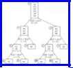
Example 8.8. Consider the insertion sort algorithm with n = 3. Suppose that initially A[1], A[2], and A[3] have key values a, b, and c, respectively. Any of the six orderings of a, b, and c could be the correct one, so we begin construction of our decision tree with the node labeled (1) in Fig. 8.23, which represents all possible orderings. The insertion sort algorithm first compares A[2] with A[1], that is, b with a. If b turns out to be the smaller, then the correct ordering can only be bac, bca, or cba, the three orderings in which b precedes a. These three orderings are represented by node (2) in Fig. 8.23. The other three orderings are represented by node (3), the right child of (1). They are the orderings for which a precedes b.

Fig. 8.23. Decision tree for insertion sort with n = 3.

Now consider what happens if the initial data is such that we reach node (2). We have just swapped A[1] with A[2], and find A[2] can rise no higher since it is at the "top" already. The current ordering of the elements is bac. Insertion sort next begins inserting A[3] into its rightful place, by comparing A[3] with A[2]. Since A[2] now holds a and A[3] holds c, we are comparing c with a; node (4) represents the two

http://www.ourstillwaters.org/stillwaters/csteaching/DataStructuresAndAlgorithms/mf1208.htm (32 of 44) [1.7.2001 19:22:21]

Data Structures and Algorithms: CHAPTER 8: Sorting

orderings from node (2) in which c precedes a, while (5) represents the one ordering where it does not.

If the algorithm reaches the status of node (5), it will end, since it has already moved A[3] as high as it can go. On the other hand in the status of node (4), we found A[3]<A[2], and so swapped them, leaving b in A[1] and c in A[2]. Insertion sort next compares these two elements and swaps them if c<b. Nodes (8) and (9) represents the orderings consistent with c<b and its opposite, respectively, as well as the information gathered going from nodes (1) to (2) to (4), namely b<a and c<a. Insertion sort ends, whether or not it has swapped A[2] with A[1], making no more comparisons. Fortunately, each of the leaves (5), (8), and (9) represent a single ordering, so we have gathered enough information to determine the correct sorted order.

The description of the tree descending from node (3) is quite symmetric with what we have seen, and we omit it. Figure 8.23, since all its leaves are associated with a single ordering, is seen to determine the correct sorted order of three key values a, b, and c.

The Size of Decision Trees

Figure 8.23 has six leaves, corresponding to the six possible orderings of the initial list a, b, c. In general, if we sort a list of n elements, there are n! = n(n - 1)(n - 2) × × ×

(2)(1) possible outcomes, which are the correct sorted orders for the initial list a1, a2,

. . . , an. That is, any of the n elements could be first, any of the remaining n - 1 second, any of the remaining n - 2 third, and so on. Thus any decision tree describing a correct sorting algorithm working on a list of n elements must have at least n! leaves, since each possible ordering must be alone at a leaf. In fact, if we delete nodes corresponding to unnecessary comparisons, and if we delete leaves that correspond to no ordering at all (since the leaves can only be reached by an inconsistent series of comparison results), there will be exactly n! leaves.

Binary trees that have many leaves must have long paths. The length of a path from the root to a leaf gives the number of comparisons made when the ordering represented by that leaf is the sorted order for a certain input list L. Thus, the length of the longest path from the root to a leaf is a lower bound on the number of steps performed by the algorithm in the worst case. Specifically, if L is the input list, the algorithm will make at least as many comparisons as the length of the path, in addition, probably, to other steps that are not comparisons of keys.

We should therefore ask how short can all paths be in a binary tree with k leaves.

http://www.ourstillwaters.org/stillwaters/csteaching/DataStructuresAndAlgorithms/mf1208.htm (33 of 44) [1.7.2001 19:22:21]

Data Structures and Algorithms: CHAPTER 8: Sorting

A binary tree in which all paths are of length p or less can have 1 root, 2 nodes at level 1, 4 nodes at level 2, and in general, 2i nodes at level i. Thus, the largest number of leaves of a tree with no nodes at levels higher than p is 2p. Put another way, a binary tree with k leaves must have a path of length at least logk. If we let k = n!, then we know that any sorting algorithm that only uses comparisons to determine the sorted order must take W(log(n!)) time in the worst case.

But how fast does log(n!) grow? A close approximation to n! is (n/e)n, where e = 2.7183 × × × is the base of natural logarithms. Since log((n/e)n) = nlogn-nloge, we see that log(n!) is on the order of nlogn. We can get a precise lower bound by noting that n(n - 1) × × × (2)(1) is the product of at least n/2 factors that are each at least n/2. Thus n! ³ (n/2)n/2. Hence log(n!) ³ (n/2)log(n/2) = (n/2)logn - n/2. Thus sorting by comparisons requires W(nlogn) time in the worst case.

The Average Case Analysis

One might wonder if there could be an algorithm that used only comparisons to sort, and took W(nlogn) time in the worst case, as all such algorithms must, but on the average took time that was O(n) or something less than O(nlogn). The answer is no, and we shall only mention how to prove the statement, leaving the details to the reader.

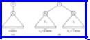
What we want to prove is that in any binary tree with k leaves, the average depth of a leaf is at least logk. Suppose that were not the case, and let tree T be the counterexample with the fewest nodes. T cannot be a single node, because our statement says of one-leaf trees only that they have average depth of at least 0. Now suppose T has k leaves. A binary tree with k ³ 2 leaves looks either like the tree in Fig. 8.24(a) or that in (b).

Fig. 8.24. Possible forms of binary tree T.

Figure 8.24(a) cannot be the smallest counterexample, because the tree rooted at n1 has as many leaves as T, but even smaller average depth. If Fig. 8.24(b) were T,

then the trees rooted at n1 and n2, being smaller then T, would not violate our claim. That is, the average depth of leaves in T1 is at least log(k1), and the average depth in

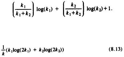
T2 is at least log(k2). Then the average depth in T is

http://www.ourstillwaters.org/stillwaters/csteaching/DataStructuresAndAlgorithms/mf1208.htm (34 of 44) [1.7.2001 19:22:21]

Data Structures and Algorithms: CHAPTER 8: Sorting

Since k1 + k2 = k, we can express the average depth as

The reader can check that when k1 = k2 = k/2, (8.13) has value logk. The reader must show that (8.13) has a minimum when k1 = k2, given the constraint that k1 + k2 = k. We leave this proof as an exercise to the reader skilled in differential calculus. Granted that (8.13) has a minimum value of logk, we see that T was not a counterexample at all.

8.7 Order Statistics

The problem of computing order statistics is, given a list of n records and an integer k, to find the key of the record that is kth in the sorted order of the records. In general, we refer to this problem as "finding the kth out of n." Special cases occur when k = 1 (finding the minimum), k = n (finding the maximum), and the case where n is odd and k = (n + 1)/2, called finding the median.

Certain cases of the problem are quite easy to solve in linear time. For example, finding the minimum of n elements in O (n) time requires no special insight. As we mentioned in connection with heapsort, if k £ n/logn then we can find the kth out of n by building a heap, which takes O (n) time, and then selecting the k smallest elements in O(n + k log n) = O(n) time. Symmetrically, we can find the kth of n in O(n) time when k ³ n - n/log n.

A Quicksort Variation

Probably the fastest way, on the average, to find the kth out of n is to use a recursive procedure similar to quicksort, call it select(i, j, k), that finds the kth element among A[i], . . . , A[j] within some larger array A [1], . . . , A [n]. The basic steps of select are:

1. Pick a pivot element, say v.

http://www.ourstillwaters.org/stillwaters/csteaching/DataStructuresAndAlgorithms/mf1208.htm (35 of 44) [1.7.2001 19:22:21]