Data-Structures-And-Algorithms-Alfred-V-Aho

Data Structures and Algorithms: CHAPTER 6: Directed Graphs

the matrix A such that A[i, j] = 1 if there is a path of length one or more from i to j, and 0 otherwise. A is often called the transitive closure of the adjacency matrix.

Example 6.10. Figure 6.20 shows the transitive closure for the adjacency matrix of the digraph of Fig. 6.14.

The transitive closure can be computed using a procedure similar to Floyd by applying the following formula in the kth pass over the boolean A matrix.

Ak[i, j] = Ak-1[i,

j] or (Ak-1[i, k] and Ak- 1[k, j])

This formula states that there is a path from i to j not passing through a

Fig. 6.20. Transitive closure.

vertex numbered higher than k if

1.there is already a path from i to j not passing through a vertex numbered higher than k- 1 or

2.there is a path from i to k not passing through a vertex numbered higher than k - 1 and a path from k to j not passing through a vertex numbered higher than k- 1.

As before Ak[i, k] = Ak-1[i, k] and Ak[k, j] = Ak-1[k, j] so we can perform the computation with only one copy of the A matrix. The resulting Pascal program, named Warshall after its discoverer, is shown in Fig. 6.21.

procedure Warshall ( var A: array[1..n, 1..n

] of boolean;

C: array[1..n, 1..n] of boolean );

{ Warshall makes A the transitive closure of C } var

http://www.ourstillwaters.org/stillwaters/csteaching/DataStructuresAndAlgorithms/mf1206.htm (15 of 31) [1.7.2001 19:12:41]

Data Structures and Algorithms: CHAPTER 6: Directed Graphs

i, j, k: integer; begin

for i := 1 to n do for j := 1 to n do

A[i, j] := C[i, j]; for k := 1 to n do

for i := 1 to n do for j := 1 to n do

if A[i, j ] = false then A[i, j] := A[i, k] and

A[k, j]

end; { Warshall }

Fig. 6.21. Warshall's algorithm for transitive closure.

An Example: Finding the Center of a

Digraph

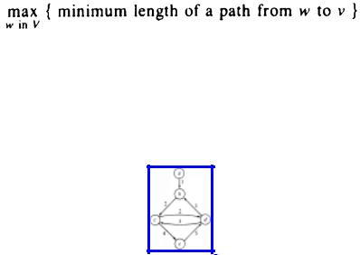
Suppose we wish to determine the most central vertex in a digraph. This problem can be readily solved using Floyd's algorithm. First, let us make more precise the term "most central vertex." Let v be a vertex in a digraph G = (V, E). The eccentricity of v is

The center of G is a vertex of minimum eccentricity. Thus, the center of a digraph is a vertex that is closest to the vertex most distant from it.

Example 6.11. Consider the weighted digraph shown in Fig. 6.22.

Fig. 6.22. Weighted digraph.

The eccentricities of the vertices are

http://www.ourstillwaters.org/stillwaters/csteaching/DataStructuresAndAlgorithms/mf1206.htm (16 of 31) [1.7.2001 19:12:41]

Data Structures and Algorithms: CHAPTER 6: Directed Graphs

vertex eccentricity

a∞

b6

c8

d5

e7

Thus the center is vertex d.

Finding the center of a digraph G is easy. Suppose C is the cost matrix for G.

1.First apply the procedure Floyd of Fig. 6.16 to C to compute the all-pairs shortest paths matrix A.

2.Find the maximum cost in each column i. This gives us the eccentricity of vertex i.

3.Find a vertex with minimum eccentricity. This is the center of G.

This running time of this process is dominated by the first step, which takes O(n3) time. Step (2) takes O(n2) time and step (3) O(n) time.

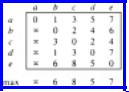
Example 6.12. The APSP cost matrix for Fig. 6.22 is shown in Fig. 6.23. The maximum value in each column is shown below.

Fig. 6.23. APSP cost matrix.

6.5 Traversals of Directed Graphs

To solve many problems dealing with directed graphs efficiently we need to visit the vertices and arcs of a directed graph in a systematic fashion. Depth-first search, a generalization of the preorder traversal of a tree, is one important technique for doing so. Depth-first search can serve as a skeleton around which many other efficient graph algorithms can be built. The last two sections of this chapter contain several algorithms that use depth-first search as a foundation.

Suppose we have a directed graph G in which all vertices are initially marked

http://www.ourstillwaters.org/stillwaters/csteaching/DataStructuresAndAlgorithms/mf1206.htm (17 of 31) [1.7.2001 19:12:41]

Data Structures and Algorithms: CHAPTER 6: Directed Graphs

unvisited. Depth-first search works by selecting one vertex v of G as a start vertex; v is marked visited. Then each unvisited vertex adjacent to v is searched in turn, using depth-first search recursively. Once all vertices that can be reached from v have been visited, the search of v is complete. If some vertices remain unvisited, we select an unvisited vertex as a new start vertex. We repeat this process until all vertices of G have been visited.

This technique is called depth-first search because it continues searching in the forward (deeper) direction as long as possible. For example, suppose x is the most recently visited vertex. Depth-first search selects some unexplored arc x → y emanating from x. If y has been visited, the procedure looks for another unexplored arc emanating from x. If y has not been visited, then the procedure marks y visited and initiates a new search at y. After completing the search through all paths beginning at y, the search returns to x, the vertex from which y was first visited. The process of selecting unexplored arcs emanating from x is then continued until all arcs from x have been explored.

An adjacency list L[v] can be used to represent the vertices adjacent to vertex v, and an array mark, whose elements are chosen from (visited, unvisited), can be used to determine whether a vertex has been previously visited. The recursive procedure dfs is outlined in Fig. 6.24. To use it on an n-vertex graph, we initialize mark to unvisited and then commence a depth-first search from each vertex that is still unvisited when its turn comes, by

for v := 1 to n do mark[v] := unvisited;

for v := 1 to n do

if mark[v] = unvisited then dfs( v )

Note that Fig. 6.24 is a template to which we shall attach other actions later, as we apply depth-first search. The code in Fig. 6.24 doesn't do anything but set the mark array.

Analysis of Depth-First Search

All the calls to dfs in the depth-first search of a graph with e arcs and n ≤ e vertices take O(e) time. To see why, observe that on no vertex is dfs called more than once, because as soon as we call dfs(v) we set mark[v] to visited at line (1), and we never call dfs on a vertex that previously had its mark set to visited. Thus, the total time spent at lines (2)-(3) going down the adjacency lists is proportional to the sum of the

http://www.ourstillwaters.org/stillwaters/csteaching/DataStructuresAndAlgorithms/mf1206.htm (18 of 31) [1.7.2001 19:12:41]

Data Structures and Algorithms: CHAPTER 6: Directed Graphs

lengths of those lists, that is, O(e). Thus, assuming n≤e, the total time spent on the depthfirst search of an entire graph is O(e), which is, to within a constant factor, the time needed merely to "look at" each arc.

(2)for each vertex w on L[v] do

Fig. 6.24. Depth-first search.

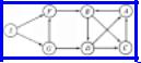
Example 6.13. Assume the procedure dfs(v) is applied to the directed graph of Fig. 6.25 with v = A. The algorithm marks A visited and selects vertex B from the adjacency list of vertex A. Since B is unvisited, the search continues by calling dfs(B). The algorithm now marks B visited and selects the first vertex from the adjacency list for vertex B. Depending on the order of the vertices on the adjacency list of B the search will go to C or D next.

Assuming that C appears ahead of D, dfs(C) is invoked. Vertex A is on the adjacency list of C. However, A is already visited at this point so the

Fig. 6.25. Directed graph.

search remains at C. Since all vertices on the adjacency list at C have now been exhausted, the search returns to B, from which the search proceeds to D. Vertices A and C on the adjacency list of D were already visited, so the search returns to B and then to A.

At this point the original call of dfs(A) is complete. However, the digraph has not been entirely searched; vertices E, F and G are still unvisited. To complete the search, we can call dfs(E).

http://www.ourstillwaters.org/stillwaters/csteaching/DataStructuresAndAlgorithms/mf1206.htm (19 of 31) [1.7.2001 19:12:41]

Data Structures and Algorithms: CHAPTER 6: Directed Graphs

The Depth-first Spanning Forest

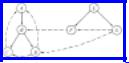
During a depth-first traversal of a directed graph, certain arcs, when traversed, lead to unvisited vertices. The arcs leading to new vertices are called tree arcs and they form a depth-first spanning forest for the given digraph. The solid arcs in Fig. 6.26 form a depth-first spanning forest for the digraph of Fig. 6.25. Note that the tree arcs must indeed form a forest, since a vertex cannot be unvisited when two different arcs to it are traversed.

In addition to the tree arcs, there are three other types of arcs defined by a depthfirst search of a directed graph. These are called back arcs, forward arcs, and cross arcs. An arc such as C → A is called a back arc, since it goes from a vertex to one of its ancestors in the spanning forest. Note that an arc from a vertex to itself is a back arc. A nontree arc that goes from a vertex to a proper descendant is called a forward arc. There are no forward arcs in Fig. 6.26.

Arcs such as D → C or G → D, which go from a vertex to another vertex that is neither an ancestor nor a descendant, are called cross arcs. Observe that all cross arcs in Fig. 6.26 go from right to left, on the assumption that we add children to the tree in the order they were visited, from left to right, and that we add new trees to the forest from left to right. This pattern is not accidental. Had the arc G → D been the arc D → G, then G would have been unvisited when the search at D was in progress, and thus on encountering arc D → G, vertex G would have been made a descendant of D, and D → G would have become a tree arc.

Fig. 6.26. Depth-first spanning forest for Fig. 6.25.

How do we distinguish among the four types of arcs? Clearly tree arcs are special since they lead to unvisited vertices during the depth-first search. Suppose we number the vertices of a directed graph in the order in which we first mark them visited during a depth-first search. That is, we may assign to an array

dfnumber [v] := count; count : = count + 1;

after line (1) of Fig. 6.24. Let us call this the depth-first numbering of a directed

http://www.ourstillwaters.org/stillwaters/csteaching/DataStructuresAndAlgorithms/mf1206.htm (20 of 31) [1.7.2001 19:12:41]

Data Structures and Algorithms: CHAPTER 6: Directed Graphs

graph; notice how depth-first numbering generalizes the preorder numbering introduced in Section 3.1.

All descendants of a vertex v are assigned depth-first search numbers greater than or equal to the number assigned v. In fact, w is a descendant of v if and only if dfnumber(v) ≤ dfnumber(w) ≤ dfnumber(v) + number of descendants of v. Thus, forward arcs go from low-numbered to high-numbered vertices and back arcs go from high-numbered to low-numbered vertices.

All cross arcs go from high-numbered vertices to low-numbered vertices. To see this, suppose that x → y is an arc and dfnumber(x) ≤ dfnumber(y). Thus x is visited before y. Every vertex visited between the time dfs(x) is first invoked and the time dfs(x) is complete becomes a descendant of x in the depth-first spanning forest. If y is unvisited at the time arc x → y is explored, x → y becomes a tree arc. Otherwise, x → y is a forward arc. Thus there can be no cross arc x → y with dfnumber (x) ≤ dfnumber (y).

In the next two sections we shall show how depthfirst search can be used in solving various graph problems.

6.6 Directed Acyclic Graphs

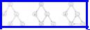
A directed acyclic graph, or dag for short, is a directed graph with no cycles. Measured in terms of the relationships they can represent, dags are more general than trees but less general than arbitrary directed graphs. Figure 6.27 gives an example of a tree, a dag, and a directed graph with a cycle.

Fig. 6.27. Three directed graphs.

Among other things, dags are useful in representing the syntactic structure of arithmetic expressions with common subexpressions. For example, Fig. 6.28 shows a dag for the expression

((a+b)*c + ((a+b)+e) * (e+f)) * ((a+b)*c)

The terms a+b and (a+b)*c are shared common subexpressions that are represented by vertices with more than one incoming arc.

http://www.ourstillwaters.org/stillwaters/csteaching/DataStructuresAndAlgorithms/mf1206.htm (21 of 31) [1.7.2001 19:12:41]

Data Structures and Algorithms: CHAPTER 6: Directed Graphs

Dags are also useful in representing partial orders. A partial order R on a set S is a binary relation such that

1.for all a in S, a R a is false (R is irreflexive)

2.for all a, b, c in S, if a R b and b R c, then a R c (R is transitive)

Two natural examples of partial orders are the "less than" (<) relation on integers, and the relation of proper containment ( ) on sets.

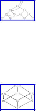
Example 6.14. Let S = {1, 2, 3} and let P(S) be the power set of S, that is, the set of all subsets of S. P(S) = {Ø, {1}, {2}, {3}, {1,2}, {1,3}, {2,3}, {1,2,3}}. is a partial order on P(S). Certainly, A A is false for any set A (irreflexivity), and if A B and B C, then A C (transitivity).

Dags can be used to portray partial orders graphically. To begin, we can view a relation R as a set of pairs (arcs) such that (a, b) is in the set if and only if a R b is true. If R is a partial order on a set S, then the directed graph G = (S ,R) is a dag. Conversely, suppose G = (S ,R) is a dag and R+ is the relation defined by a R+ b if and only if there is a path of length one or

Fig. 6.28. Dag for arithmetic expression.

more from a to b. (R+ is the transitive closure of the relation R.) Then, R+ is a partial order on S.

Example 6.15. Figure 6.29 shows a dag (P(S), R), where S = {1, 2 ,3}. The relation R+ is proper containment on the power set P(S).

Fig. 6.29. Dag of proper containments.

http://www.ourstillwaters.org/stillwaters/csteaching/DataStructuresAndAlgorithms/mf1206.htm (22 of 31) [1.7.2001 19:12:41]

Data Structures and Algorithms: CHAPTER 6: Directed Graphs

Test for Acyclicity

Suppose we are given a directed graph G = (V, E), and we wish to determine whether G is acyclic, that is, whether G has no cycles. Depth-first search can be used to answer this question. If a back arc is encountered during a depth-first search of G, then clearly the graph has a cycle. Conversely, if a directed graph has a cycle, then a back arc will always be encountered in any depth-first search of the graph.

To see this fact, suppose G is cyclic. If we do a depth-first search of G, there will be one vertex v having the lowest depth-first search number of any vertex on a cycle. Consider an arc u → v on some cycle containing v. Since u is on the cycle, u must be a descendant of v in the depth-first spanning forest. Thus, u → v cannot be a cross arc. Since the depthfirst number of u is greater than the depth-first number of v, u → v cannot be a tree arc or a forward arc. Thus, u → v must be a back arc, as illustrated in Fig. 6.30.

Fig. 6.30. Every cycle contains a back arc.

Topological Sort

A large project is often divided into a collection of smaller tasks, some of which have to be performed in certain specified orders so that we may complete the entire project. For example, a university curriculum may have courses that require other courses as prerequisites. Dags can be used to model such situations naturally. For example, we could have an arc from course C to course D if C is a prerequisite for D.

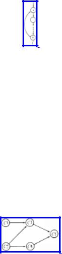
Example 6.16. Figure 6.31 shows a dag giving the prerequisite structure on five courses. Course C3, for example, requires courses C1 and C2 as prerequisites.

Fig. 6.31. Dag of prerequisites.

http://www.ourstillwaters.org/stillwaters/csteaching/DataStructuresAndAlgorithms/mf1206.htm (23 of 31) [1.7.2001 19:12:41]

Data Structures and Algorithms: CHAPTER 6: Directed Graphs

Topological sort is a process of assigning a linear ordering to the vertices of a dag so that if there is an arc from vertex i to vertex j, then i appears before j in the linear ordering. For example, C1, C2, C3, C4, C5 is a topological sort of the dag in Fig. 6.31. Taking the courses in this sequence would satisfy the prerequisite structure given in Fig. 6.31.

Topological sort can be easily accomplished by adding a print statement after line (4) to the depth-first search procedure in Fig. 6.24:

procedure topsort ( v: vertex );

{ print vertices accessible from v in reverse topological order }

var

w: vertex;

begin

mark[v] := visited;

for each vertex w on L[v] do

if mark[w] = unvisited then

topsort(w) ;

writeln(v)

end; { topsort }

When topsort finishes searching all vertices adjacent to a given vertex x, it prints x. The effect of calling topsort (v) is to print in a reverse topological order all vertices of a dag accessible from v by a path in the dag.

This technique works because there are no back arcs in a dag. Consider what happens when depth-first search leaves a vertex x for the last time. The only arcs emanating from v are tree, forward, and cross arcs. But all these arcs are directed towards vertices that have already been completely visited by the search and therefore precede x in the order being constructed.

http://www.ourstillwaters.org/stillwaters/csteaching/DataStructuresAndAlgorithms/mf1206.htm (24 of 31) [1.7.2001 19:12:41]