Data-Structures-And-Algorithms-Alfred-V-Aho

Data Structures and Algorithms: CHAPTER 5: Advanced Set Representation Methods

with relatively little effort.

Unfortunately, it is very difficult to analyze the average cost of FIND's when path compression is used. It turns out that if we do not require that smaller trees be merged into larger ones, we require no more than O(n log n) time to do n FIND's. Of course, the first FIND may take O(n) time by itself for a tree consisting of one chain. But path compression can change a tree very rapidly and no matter in what order we apply FIND to elements of any tree no more than O(n) time is spent on n FIND's. However, there are

Fig. 5.24. Example of the MFSET data structure.

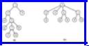
Fig. 5.25. MFSET represented by a collection of trees.

sequences of MERGE and FIND instructions that require Ω(nlog n) time.

The algorithm that both uses path compression and merges the smaller tree into the larger is asymptotically the most efficient method known for implementing MFSET's. In particular, n FIND's require no more than O(nα(n)) time, where α(n) is a function that is not constant, yet grows much more slowly than logn. We shall define α(n) below, but the analysis that leads to this bound is beyond the scope of this book.

Fig. 5.26. Merging B into A.

http://www.ourstillwaters.org/stillwaters/csteaching/DataStructuresAndAlgorithms/mf1205.htm (35 of 47) [1.7.2001 19:09:32]

Data Structures and Algorithms: CHAPTER 5: Advanced Set Representation Methods

Fig. 5.27. An example of path compression.

The Function α(n)

The function a(n) is closely related to a very rapidly growing function A(x, y), known as Ackermann's function. A(x, y) is defined recursively by:

A(0,y) = 1 for y ³ 0

A(1, 0) = 2

A(x, 0) = x+2 for x ³ 2

A(x,y) = A(A(x-1, y),y-1) for x, y ³ 1

Each value of y defines a function of one variable. For example, the third line above tells us that for y=0, this function is "add 2." For y = 1, we have A(x, 1) = A(A(x-1, 1),0) = A(x-1, 1) + 2, for x > 1, with A(1, 1) = A(A(0, 1),0) = A(1, 0) = 2. Thus A(x, 1) = 2x for all x ³ 1. In other words, A(x, 1) is "multiply by 2." Then, A(x, 2) = A(A(x-1, 2), 1) = 2A(x-1, 2) for x > 1. Also, A(1, 2) = A(A(0,2), 1) = A(1, 1) = 2. Thus A(x, 2) = 2x. Similarly, we can show that A(x, 3) = 22...2 (stack of x 2's), while A(x, 4) is so rapidly growing there is no accepted mathematical notation for such a function.

A single-variable Ackermann's function can be defined by letting A(x) = A(x, x). The function a(n) is a pseudo-inverse of this single variable function. That is, a(n) is the least x such that n £ A(x). For example, A(1) = 2, so a(1) = a(2) = 1. A(2) = 4, so a(3) = a(4) = 2. A(3) = 8, so a(5) = . . . = a(8) = 3. So far, a(n) seems to be growing rather steadily.

However, A(4) is a stack of 65536 2's. Since log(A(4)) is a stack of 65535 2's, we cannot hope even to write A(4) explicitly, as it would take log(A(4)) bits to do so. Thus a(n) £ 4 for all integers n one is ever likely to encounter. Nevertheless, a(n) eventually reaches 5, 6, 7, . . . on its unimaginably slow course toward infinity.

5.6 An ADT with MERGE and SPLIT

http://www.ourstillwaters.org/stillwaters/csteaching/DataStructuresAndAlgorithms/mf1205.htm (36 of 47) [1.7.2001 19:09:32]

Data Structures and Algorithms: CHAPTER 5: Advanced Set Representation Methods

Let S be a set whose members are ordered by the relation <. The operation SPLIT(S, S1, S2, x) partitions S into two sets: S1={ a ½ a is in S and a < x} and S2 = {a ½ a is in

S and a ³ x}. The value of S after the split is undefined, unless it is one of S1 or S2. There are several situations where the operation of splitting sets by comparing each member with a fixed value x is essential. We shall consider one such problem here.

The Longest Common Subsequence

Problem

A subsequence of a sequence x is obtained by removing zero or more (not necessarily contiguous) elements from x. Given two sequences x and y, a longest common subsequence (LCS) is a longest sequence that is a subsequence of both x and y.

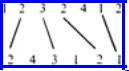
For example, an LCS of 1, 2, 3, 2, 4, 1, 2 and 2, 4, 3, 1, 2, 1 is the subsequence 2, 3, 2, 1, formed as shown in Fig. 5.28. There are other LCS's as well, such as 2, 4, 1, 2, but there are no common subsequences of length 5.

Fig. 5.28. A longest common subsequence.

There is a UNIX command called diff that compares files line-by-line, finding a longest common subsequence, where a line of a file is considered an element of the subsequence. That is, whole lines are analogous to the integers 1, 2, 3, and 4 in Fig. 5.28. The assumption behind the command diff is that the lines of each file that are not in this LCS are lines inserted, deleted or modified in going from one file to the other. For example, if the two files are versions of the same program made several days apart, diff will, with high probability, find the changes.

There are several general solutions to the LCS problem that work in O(n2) steps on sequences of length n. The command diff uses a different strategy that works well when the files do not have too many repetitions of any line. For example, programs will tend to have lines "begin" and "end" repeated many times, but other lines are not likely to repeat.

The algorithm used by diff for finding an LCS makes use of an efficient implementation of sets with operations MERGE and SPLIT, to work in time

http://www.ourstillwaters.org/stillwaters/csteaching/DataStructuresAndAlgorithms/mf1205.htm (37 of 47) [1.7.2001 19:09:32]

Data Structures and Algorithms: CHAPTER 5: Advanced Set Representation Methods

O(plogn), where n is the maximum number of lines in a file and p is the number of pairs of positions, one from each file, that have the same line. For example, p for the strings in Fig. 5.28 is 12. The two 1's in each string contribute four pairs, the 2's contribute six pairs, and 3 and 4 contribute one pair each. In the worst case, p,. could be n2, and this algorithm would take O(n2logn) time. However, in practice, p is usually closer to n, so we can expect an O(nlogn) time complexity.

To begin the description of the algorithm let A = a1a2 × × × an and B = b1b2 × × × bm be the two strings whose LCS we desire. The first step is to tabulate for each value a, the positions of the string A at which a appears. That is, we define PLACES(a)= { i ½ a = ai }. We can compute the sets PLACES(a) by constructing a mapping from symbols to headers of lists of positions. By using a hash table, we can create the sets PLACES(a) in O(n) "steps" on the average, where a "step" is the time it takes to operate on a symbol, say to hash it or compare it with another. This time could be a constant if symbols are characters or integers, say. However, if the symbols of A and B are really lines of text, then steps take an amount of time that depends on the average length of a line of text.

Having computed PLACES(a) for each symbol a that occurs in string A, we are ready to find an LCS. To simplify matters, we shall only show how to find the length of the LCS, leaving the actual construction of the LCS as an exercise. The algorithm considers each bj, for j = 1, 2, ... , m, in turn. After considering bj, we need to know,

for each i between 0 and n, the length of the LCS of strings a1 × × × ai and b1 × × × bj.

We shall group values of i into sets Sk, for k = 0, 1, . . . , n, where Sk consists of all those integers i such that the LCS of a1 × × × ai and b1 × × × bj has length k. Note that Sk will always be a set of consecutive integers, and the integers in Sk+1 are larger than those in Sk, for all k.

Example 5.8. Consider Fig. 5.28, with j = 5. If we try to match zero symbols from the first string with the first five symbols of the second (24312), we naturally have an LCS of length 0, so 0 is in S0. If we use the first symbol from the first string, we can obtain an LCS of length 1, and if we use the first two symbols, 12, we can obtain an LCS of length 2. However, using 123, the first three symbols, still gives us an LCS of length 2 when matched against 24312. Proceeding in this manner, we discover S0 = {0}, S1 = {1}, S2 = {2, 3}, S3 = {4, 5, 6}, and S4 = {7}.

Suppose that we have computed the Sk's for position j-1 of the second string and we wish to modify them to apply to position j. We consider the set PLACES(bj). For each r in PLACES(bj), we consider whether we can improve some of the LCS's by

http://www.ourstillwaters.org/stillwaters/csteaching/DataStructuresAndAlgorithms/mf1205.htm (38 of 47) [1.7.2001 19:09:32]

Data Structures and Algorithms: CHAPTER 5: Advanced Set Representation Methods

adding the match between ar and bj to the LCS of a1 × × × ar- 1 and b1 × × × bj. That is, if both r-1 and r are in Sk, then all s ³ r in Sk really belong in Sk+1 when bj is considered. To see this we observe that we can obtain k matches between a1 × × × ar-1 and bl × × × bj-1, to which we add a match between ar and bj. We can modify Sk and

Sk+1 by the following steps.

1.FIND(r) to get Sk.

2.If FIND(r-1) is not Sk, then no benefit can be had by matching bj with ar. Skip the remaining steps and do not modify Sk or Sk+1.

3.If FIND(r-1) = Sk, apply SPLIT(Sk, Sk, S'k, r) to separate from Sk those members greater than or equal to r.

4.MERGE(S'k, Sk+1, Sk+1) to move these elements into Sk+1.

It is important to consider the members of PLACES(bj) largest first. To see why, suppose for example that 7 and 9 are in PLACES(bj), and before bj is considered,

S3={6, 7, 8, 9} and S4={10, 11}.

If we consider 7 before 9, we split S3 into S3 = {6} and S'3 = {7, 8, 9}, then make

S4 = {7, 8, 9, 10, 11}. If we then consider 9, we split S4 into S4={7, 8} and S'4 = {9, 10, 11}, then merge 9, 10 and 11 into S5. We have thus moved 9 from S3 to S5 by considering only one more position in the second string, representing an impossibility. Intuitively, what has happened is that we have erroneously matched bj against both a7 and a9 in creating an imaginary LCS of length 5.

In Fig. 5.29, we see a sketch of the algorithm that maintains the sets Sk as we scan the second string. To determine the length of an LCS, we need only execute FIND(n) at the end.

procedure LCS; begin

(1)initialize S0 = {0, 1, ... , n} and Si = - for i = 1, 2, ... , n;

(2)for j := 1 to n do { compute Sk's for position

j }

(3)for r in PLACES(bj), largest first do begin

smallest in Sk }

http://www.ourstillwaters.org/stillwaters/csteaching/DataStructuresAndAlgorithms/mf1205.htm (39 of 47) [1.7.2001 19:09:33]

Data Structures and Algorithms: CHAPTER 5: Advanced Set Representation Methods

end end

end; { LCS }

Fig. 5.29. Sketch of longest common subsequence program.

Time Analysis of the LCS Algorithm

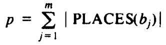
As we mentioned earlier, the algorithm of Fig. 5.29 is a useful approach only if there are not too many matches between symbols of the two strings. The measure of the number of matches is

where |PLACES(bj)| denotes the number of elements in set PLACES(bj). In other words, p is the sum over all bj of the number of positions in the first string that match bj. Recall that in our discussion of file comparison, we expect p to be of the same order as m and n, the lengths of the two strings (files).

It turns out that the 2-3 tree is a good structure for the sets Sk. We can initialize these sets, as in line (1) of Fig. 5.29, in O(n) steps. The FIND operation requires an array to serve as a mapping from positions r to the leaf for r and also requires pointers to parents in the 2-3 tree. The name of the set, i.e., k for Sk, can be kept at the root, so we can execute FIND in O(logn) steps by following parent pointers until we reach the root. Thus all executions of lines (4) and (5) together take O(plogn) time, since those lines are each executed exactly once for each match found.

The MERGE operation of line (5) has the special property that every member of S'k is lower than every member of Sk+1, and we can take advantage of this fact when using 2-3 trees for an implementation.† To begin the MERGE, place the 2-3 tree for S'k to the left of that for Sk+1. If both are of the same height, create a new root with the roots of the two trees as children. If S'k is shorter, insert the root of that tree as the

http://www.ourstillwaters.org/stillwaters/csteaching/DataStructuresAndAlgorithms/mf1205.htm (40 of 47) [1.7.2001 19:09:33]

Data Structures and Algorithms: CHAPTER 5: Advanced Set Representation Methods

leftmost child of the leftmost node of Sk+1 at the appropriate level. If this node now has four children, we modify the tree exactly as in the INSERT procedure of Fig. 5.20. An example is shown in Fig. 5.30. Similarly, if Sk+1 is shorter, make its root the rightmost child of the rightmost node of S'k at the appropriate level.

Fig. 5.30. Example of MERGE.

The SPLIT operation at r requires that we travel up the tree from leaf r, duplicating every interior node along the path and giving one copy to each of the two resulting trees. Nodes with no children are eliminated, and nodes with one child are removed and have that child inserted into the proper tree at the proper level.

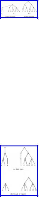
Example 5.9. Suppose we split the tree of Fig. 5.30(b) at node 9. The two trees, with duplicated nodes, are shown in Fig. 5.31(a). On the left, the parent of 8 has only one child, so 8 becomes a child of the parent of 6 and 7. This parent now has three children, so all is as it should be; if it had four children, a new node would have been created and inserted into the tree. We need only eliminate nodes with zero children (the old parent of 8) and the chain of nodes with one child leading to the root. The parent of 6, 7, and 8 becomes the new root, as shown in Fig. 5.31(b). Similarly, in the right-hand tree, 9 becomes a sibling of 10 and 11, and unnecessary nodes are eliminated, as is also shown in Fig. 5.31(b).

Fig. 5.31. An example of SPLIT.

If we do the splitting and reorganization of the 2-3 tree bottom up, it can be shown by consideration of a large number of cases that O(logn) steps suffices. Thus, the total time spent in lines (6) and (7) of Fig. 5.29 is O(plogn), and hence the entire algorithm takes O(plogn) steps. We must add in the preprocessing time needed to compute and sort PLACES(a) for symbols a. As we mentioned, if the symbols a are "large"

http://www.ourstillwaters.org/stillwaters/csteaching/DataStructuresAndAlgorithms/mf1205.htm (41 of 47) [1.7.2001 19:09:33]

Data Structures and Algorithms: CHAPTER 5: Advanced Set Representation Methods

objects, this time can be much greater than any other part of the algorithm. As we shall see in Chapter 8, if the symbols can be manipulated and compared in single "steps," then O(nlogn) time suffices to sort the first string a1a2 × × × an (actually, to sort objects (i, ai) on the second field), whereupon PLACES(a) can be read off from this list in O(n) time. Thus, the length of the LCS can be computed in O(max(n, p) logn) time which, since p ³ n is normal, can be taken as O(plogn).

Exercises

5.1

Draw all possible binary search trees containing the four elements 1, 2, 3, 4.

5.2

Insert the integers 7, 2, 9, 0, 5, 6, 8, 1 into a binary search tree by repeated application of the procedure INSERT of Fig. 5.3.

5.3Show the result of deleting 7, then 2 from the final tree of Exercise 5.2.

When deleting two elements from a binary search tree using the *5.4 procedure of Fig. 5.5, does the final tree ever depend on the order in

which you delete them?

We wish to keep track of all 5-character substrings that occur in a given

5.5string, using a trie. Show the trie that results when we insert the 14 substrings of length five of the string ABCDABACDEBACADEBA.

To implement Exercise 5.5, we could keep a pointer at each leaf, which, say, represents string abcde, to the interior node representing the suffix bcde. That way, if the next symbol, say f, is received, we don't have to

*5.6

insert all of bcdef, starting at the root. Furthermore, having seen abcde, we may as well create nodes for bcde, cde, de, and e, since we shall, unless the sequence ends abruptly, need those nodes eventually. Modify the trie data structure to maintain such pointers, and modify the trie insertion algorithm to take advantage of this data structure.

5.7

Show the 2-3 tree that results if we insert into an empty set, represented as a 2-3 tree, the elements 5, 2, 7, 0, 3, 4, 6, 1, 8, 9.

5.8

Show the result of deleting 3 from the 2-3 tree that results from Exercise 5.7.

http://www.ourstillwaters.org/stillwaters/csteaching/DataStructuresAndAlgorithms/mf1205.htm (42 of 47) [1.7.2001 19:09:33]

Data Structures and Algorithms: CHAPTER 5: Advanced Set Representation Methods

Show the successive values of the various Si's when implementing the

5.9LCS algorithm of Fig. 5.29 with first string abacabada, and second string bdbacbad.

Suppose we use 2-3 trees to implement the MERGE and SPLIT operations as in Section 5.6.

5.10a. Show the result of splitting the tree of Exercise 5.7 at 6.

b.Merge the tree of Exercise 5.7 with the tree consisting of leaves for elements 10 and 11.

Some of the structures discussed in this chapter can be modified easily to support the MAPPING ADT. Write procedures MAKENULL, ASSIGN, and COMPUTE to operate on the following data structures.

5.11a. Binary search trees. The "<" ordering applies to domain elements.

b.2-3 trees. At interior nodes, place only the key field of domain elements.

5.12

Show that in any subtree of a binary search tree, the minimum element is at a node without a left child.

5.13Use Exercise 5.12 to produce a nonrecursive version of DELETE-MIN.

5.14

Write procedures ASSIGN, VALUEOF, MAKENULL and GETNEW for trie nodes represented as lists of cells.

How do the trie (list of cells implementation), the open hash table, and *5.15 the binary search tree compare for speed and for space utilization when

elements are strings of up to ten characters?

If elements of a set are ordered by a "<" relation, then we can keep one

*5.16

or two elements (not just their keys) at interior nodes of a 2-3 tree, and we then do not have to keep these elements at the leaves. Write INSERT and DELETE procedures for 2-3 trees of this type.

http://www.ourstillwaters.org/stillwaters/csteaching/DataStructuresAndAlgorithms/mf1205.htm (43 of 47) [1.7.2001 19:09:33]

Data Structures and Algorithms: CHAPTER 5: Advanced Set Representation Methods

Another modification we could make to 2-3 trees is to keep only keys at interior nodes, but do not require that the keys k1 and k2 at a node truly be the minimum keys of the second and third subtrees, just that all keys k of the third subtree satisfy k ³ k2, all keys k of the second satisfy k1 £ k

< k2, and all keys k of the first satisfy k < k1.

5.17

a.How does this convention simplify the DELETE operation?

b.Which of the dictionary and mapping operations are made more complicated or less efficient?

Another data structure that supports dictionaries with the MIN operation is the AVL tree (named for the inventors' initials) or height-balanced

*5.18

tree. These trees are binary search trees in which the heights of two siblings are not permitted to differ by more than one. Write procedures to implement INSERT and DELETE, while maintaining the AVL-tree property.

5.19Write the Pascal program for procedure delete1 of Fig. 5.21.

A finite automaton consists of a set of states, which we shall take to be the integers 1..n and a table transitions[state, input] giving a next state for each state and each input character. For our purposes, we shall assume that the input is always either 0 or 1. Further, certain of the states

are designated accepting states. For our purposes, we shall assume that all and only the even numbered states are accepting. Two states p and q

*5.20 are equivalent if either they are the same state, or (i) they are both accepting or both nonaccepting, (ii) on input 0 they transfer to equivalent states, and (iii) on input 1 they transfer to equivalent states. Intuitively, equivalent states behave the same on all sequences of inputs; either both or neither lead to accepting states. Write a program using the MFSET operations that computes the sets of equivalent states of a given finite automaton.

http://www.ourstillwaters.org/stillwaters/csteaching/DataStructuresAndAlgorithms/mf1205.htm (44 of 47) [1.7.2001 19:09:33]