Data-Structures-And-Algorithms-Alfred-V-Aho

Data Structures and Algorithms: CHAPTER 7: Undirected Graphs

To build progressively larger components, we examine edges from E, in order of increasing cost. If the edge connects two vertices in two different connected components, then we add the edge to T. If the edge connects two vertices in the same component, then we discard the edge, since it would cause a cycle if we added it to the spanning tree for that connected component. When all vertices are in one component, T is a minimum-cost spanning tree for G.

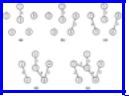
Example 7.5. Consider the weighted graph of Fig. 7.4(a). The sequence of edges added to T is shown in Fig. 7.9. The edges of cost 1, 2, 3, and 4 are considered first, and all are accepted, since none of them causes a cycle. The edges (1, 4) and (3, 4) of cost 5 cannot be accepted, because they connect vertices in the same component in Fig. 7.9(d), and therefore would complete a cycle. However, the remaining edge of cost 5, namely (2, 3), does not create a cycle. Once it is accepted, we are done.

We can implement this algorithm using sets and set operations discussed in Chapters 4 and 5. First, we need a set consisting of the edges in E. We then apply the DELETEMIN operator repeatedly to this set to select edges in order of increasing cost. The set of edges therefore forms a priority queue, and a partially ordered tree is an appropriate data structure to use here.

We also need to maintain a set of connected components C. The operations we apply to it are:

1.MERGE(A, B, C) to merge the components A and B in C and to call the result either A or B arbitrarily.†

2.FIND(v, C) to return the name of the component of C of which vertex v is a member. This operation will be used to determine whether the two vertices of an edge are in the same or different components.

3.INITIAL(A, v, C) to make A the name of a component in C containing only vertex v initially.

These are the operations of the MERGE-FIND ADT called MFSET, which we encountered in Section 5.5. A sketch of a program called Kruskal to find a minimumcost spanning tree using these operations is shown in Fig. 7.10.

We can use the techniques of Section 5.5 to implement the operations used in this program. The running time of this program is dependent on two factors. If there are e edges, it takes O(eloge) time to insert the edges into the priority queue.‡ In each iteration of the while-loop, finding the least cost

http://www.ourstillwaters.org/stillwaters/csteaching/DataStructuresAndAlgorithms/mf1207.htm (8 of 22) [1.7.2001 19:15:36]

Data Structures and Algorithms: CHAPTER 7: Undirected Graphs

Fig. 7.9. Sequence of edges added by Kruskal's algorithm.

edge in edges takes O(log e) time. Thus, the priority queue operations take O(e log e) time in the worst case. The total time required to perform the MERGE and FIND operations depends on the method used to implement the MFSET. As shown in Section 5.5, there are O(e log e) and O(e α (e)) methods. In either case, Kruskal's algorithm can be implemented to run in O(e log e) time.

7.3 Traversals

In a number of graph problems, we need to visit the vertices of a graph systematically. Depth-first search and breadth-first search, the subjects of this section, are two important techniques for doing this. Both techniques can be used to determine efficiently all vertices that are connected to a given vertex.

procedure Kruskal ( V: SET of vertex; E: SET of edges;

var T: SET of edges ); var

ncomp: integer; { current number of components } edges: PRIORITYQUEUE; { the set of edges } components: MFSET; { the set V grouped into

a MERGE-FIND set of components } u, v: vertex;

e: edge;

nextcomp: integer; { name for new component } ucomp, vcomp: integer; { component names }

begin

MAKENULL(T); MAKENULL(edges); nextcomp := 0;

ncomp := number of members of V; for v in V do begin { initialize a

component to contain one vertex of V } nextcomp := nextcomp + 1;

http://www.ourstillwaters.org/stillwaters/csteaching/DataStructuresAndAlgorithms/mf1207.htm (9 of 22) [1.7.2001 19:15:36]

Data Structures and Algorithms: CHAPTER 7: Undirected Graphs

INITIAL( nextcomp, v, components) end;

for e in E do { initialize priority queue of edges } INSERT(e, edges);

while ncomp > 1 do begin { consider next edge } e := DELETEMIN(edges);

let e = (u, v);

ucomp := FIND(u, components); vcomp := FIND(v, components); if ucomp <> vcomp then begin

{ e connects two different components } MERGE (ucomp, vcomp, components); ncomp := ncomp - 1;

INSERT(e, T) end

end

end; { Kruskal }

Fig. 7.10. Kruskal's algorithm.

Depth-First Search

Recall from Section 6.5 the algorithm dfs for searching a directed graph. The same algorithm can be used to search undirected graphs, since the undirected edge (v, w) may be thought of as the pair of directed edges v → w and w → v.

In fact, the depth-first spanning forests constructed for undirected graphs are even simpler than for digraphs. We should first note that each tree in the forest is one connected component of the graph, so if a graph is connected, it has only one tree in its depth-first spanning forest. Second, for digraphs we identified four kinds of arcs: tree, forward, back, and cross. For undirected graphs there are only two kinds: tree edges and back edges.

Because there is no distinction between forward edges and backward edges for undirected graphs, we elect to refer to them all as back edges. In an undirected graph, there can be no cross edges, that is, edges (v, w) where v is neither an ancestor nor descendant of w in the spanning tree. Suppose there were. Then let v be a vertex that is reached before w in the search. The call to dfs(v) cannot end until w has been searched, so w is entered into the tree as some descendant of v. Similarly, if dfs(w) is called before dfs(v), then v becomes a descendant of w.

http://www.ourstillwaters.org/stillwaters/csteaching/DataStructuresAndAlgorithms/mf1207.htm (10 of 22) [1.7.2001 19:15:36]

Data Structures and Algorithms: CHAPTER 7: Undirected Graphs

As a result, during a depth-first search of an undirected graph G, all edges become either

1.tree edges, those edges (v, w) such that dfs(v) directly calls dfs(w) or vice versa, or

2.back edges, those edges (v, w) such that neither dfs(v) nor dfs(w) called the other directly, but one called the other indirectly (i.e., dfs(w) calls dfs (x), which calls dfs (v), so w is an ancestor of v).

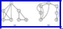
Example 7.6. Consider the connected graph G in Fig. 7.11(a). A depth-first spanning tree T resulting from a depth-first search of G is shown in Fig. 7.11(b). We assume the search began at vertex a, and we have adopted the convention of showing tree edges solid and back edges dashed. The tree has been drawn with the root on the top and the children of each vertex have been drawn in the left-to-right order in which they were first visited in the procedure of dfs.

To follow a few steps of the search, the procedure dfs(a) calls dfs(b) and adds edge (a, b) to T since b is not yet visited. At b, dfs calls dfs(d) and adds edge (b, d) to T. At d, dfs calls dfs(e) and adds edge (d, e) to T. At e, vertices a, b, and d are marked visited so dfs(e) returns without adding any edges to T. At d, dfs now sees that vertices a and b are marked visited so dfs(d) returns without adding any more edges to T. At b, dfs now sees that the remaining adjacent vertices a and e are marked visited, so dfs(b) returns. The search then continues to c, f, and g.

Fig. 7.11. A graph and its depth-first search.

Breadth-First Search

Another systematic way of visiting the vertices is called breadth-first search. The approach is called "breadth-first" because from each vertex v that we visit we search as broadly as possible by next visiting all the vertices adjacent to v. We can also apply this strategy of search to directed graphs.

As for depth-first search, we can build a spanning forest when we perform a breadth-first search. In this case, we consider edge (x, y) a tree edge if vertex y is first visited from vertex x in the inner loop of the search procedure bfs of Fig. 7.12.

http://www.ourstillwaters.org/stillwaters/csteaching/DataStructuresAndAlgorithms/mf1207.htm (11 of 22) [1.7.2001 19:15:36]

Data Structures and Algorithms: CHAPTER 7: Undirected Graphs

It turns out that for the breadth-first search of an undirected graph, every edge that is not a tree edge is a cross edge, that is, it connects two vertices neither of which is an ancestor of the other.

The breadth-first search algorithm given in Fig. 7.12 inserts the tree edges into a set T, which we assume is initially empty. Every entry in the array mark is assumed to be initialized to the value unvisited; Figure 7.12 works on one connected component. If the graph is not connected, bfs must be called on a vertex of each component. Note that in a breadth-first search we must mark a vertex visited before enqueuing it, to avoid placing it on the queue more than once.

Example 7.7. The breadth-first spanning tree for the graph G in Fig. 7.11(a) is shown in Fig. 7.13. We assume the search began at vertex a. As before, we have shown tree edges solid and other edges dashed. We have also drawn the tree with the root at the top and the children in the left-to-right order in which they were first visited.

The time complexity of breadth-first search is the same as that of depth-

procedure bfs ( v );

{ bfs visits all vertices connected to v using breadth-first search } var

Q: QUEUE of vertex; x, y: vertex;

begin

mark[v] := visited; ENQUEUE(v, Q);

while not EMPTY(Q) do begin x := FRONT(Q); DEQUEUE(Q);

for each vertex y adjacent to x do if mark[y] = unvisited then begin

mark[y] := visited; ENQUEUE(y, Q); INSERT((x, y), T)

end end

end; { bfs }

Fig. 7.12. Breadth-first search.

http://www.ourstillwaters.org/stillwaters/csteaching/DataStructuresAndAlgorithms/mf1207.htm (12 of 22) [1.7.2001 19:15:36]

Data Structures and Algorithms: CHAPTER 7: Undirected Graphs

Fig. 7.13. Breadth-first search of G.

first search. Each vertex visited is placed in the queue once, so the body of the while loop is executed once for each vertex. Each edge (x, y) is examined twice, once from x and once from y. Thus, if a graph has n vertices and e edges, the running time of bfs is O(max(n, e)) if we use an adjacency list representation for the edges. Since e ³ n is typical, we shall usually refer to the running time of breadth-first search as O(e), just as we did for depth-first search.

Depth-first search and breadth-first search can be used as frameworks around which to design efficient graph algorithms. For example, either method can be used to find the connected components of a graph, since the connected components are the trees of either spanning forest.

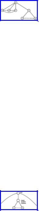
We can test for cycles using breadth-first search in O(n) time, where n is the number of vertices, independent of the number of edges. As we discussed in Section 7.1, any graph with n vertices and n or more edges must have a cycle. However, a graph could have n-1 or fewer edges and still have a cycle, if it had two or more connected components. One sure way to find the cycles is to build a breadth-first spanning forest. Then, every cross edge (v, w) must complete a simple cycle with the tree edges leading to v and w from their closest common ancestor, as shown in Fig. 7.14.

Fig. 7.14 A cycle found by breadth-first search.

7.4 Articulation Points and Biconnected

Components

An articulation point of a graph is a vertex v such that when we remove v and all edges incident upon v, we break a connected component of the graph into two or more pieces. For example, the articulation points of Fig. 7.11(a) are a and c. If we delete a, the graph, which is one connected component, is divided into two triangles:

http://www.ourstillwaters.org/stillwaters/csteaching/DataStructuresAndAlgorithms/mf1207.htm (13 of 22) [1.7.2001 19:15:36]

Data Structures and Algorithms: CHAPTER 7: Undirected Graphs

{b, d, e} and {c, f, g}. If we delete c, we divide the graph into {a, b, d, e} and {f, g}. However, if we delete any one of the other vertices from the graph of Fig. 7.11(a), we do not split the connected component. A connected graph with no articulation points is said to be biconnected. Depth-first search is particularly useful in finding the biconnected components of a graph.

The problem of finding articulation points is the simplest of many important problems concerning the connectivity of graphs. As an example of applications of connectivity algorithms, we may represent a communication network as a graph in which the vertices are sites to be kept in communication with one another. A graph has connectivity k if the deletion of any k-1 vertices fails to disconnect the graph. For example, a graph has connectivity two or more if and only if it has no articulation points, that is, if and only if it is biconnected. The higher the connectivity of a graph, the more likely the graph is to survive the failure of some of its vertices, whether by failure of the processing units at the vertices or external attack.

We shall here give a simple depth-first search algorithm to find all the articulation points of a connected graph, and thereby test by their absence whether the graph is biconnected.

1.Perform a depth-first search of the graph, computing dfnumber [v] for each vertex v as discussed in Section 6.5. In essence, dfnumber orders the vertices as in a preorder traversal of the depth-first spanning tree.

2.For each vertex v, compute low [v], which is the smallest dfnumber of v or of any vertex w reachable from v by following down zero or more tree edges to a descendant x of v (x may be v) and then following a back edge (x, w). We compute low [v] for all vertices v by visiting the vertices in a postorder traversal. When we process v, we have computed low [y] for every child y of v. We take low [v] to be the minimum of

a.dfnumber [v],

b.dfnumber [z] for any vertex z for which there is a back edge (v, z) and

c.low [y] for any child y of v.

●Now we find the articulation points as follows.

a.The root is an articulation point if and only if it has two or more children. Since there are no cross edges, deletion of the root must disconnect the subtrees rooted at its children, as a

http://www.ourstillwaters.org/stillwaters/csteaching/DataStructuresAndAlgorithms/mf1207.htm (14 of 22) [1.7.2001 19:15:36]

Data Structures and Algorithms: CHAPTER 7: Undirected Graphs

disconnects {b, d, e} from {c, f, g} in Fig. 7.11(b).

b.A vertex v other than the root is an articulation point if and only if there is some child w of v such that low [w] ³ dfnumber [v]. In

this case, v disconnects w and its descendants from the rest of the graph. Conversely, if low [w] < dfnumber [v], then there must be a way to get from w down the tree and back to a proper ancestor of v (the vertex whose dfnumber is low [w]), and therefore deletion of v does not disconnect w or its descendants from the rest of the graph.

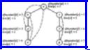
Example 7.8. dfnumber and low are computed for the graph of Fig. 7.11(a) in Fig. 7.15. As an example of the calculation of low, our postorder traversal visits e first. At e, there are back edges (e, a) and (e, b), so low [e] is set to min(dfnumber [e], dfnumber [a], dfnumber [b]) = 1. Then d is visited, and low [d] is set to the minimum of dfnumber [d], low [e], and dfnumber [a ]. The second of these arises because e is a child of d and the third because of the back edge (d, a).

Fig. 7.15. Depth-first and low numberings.

After computing low we consider each vertex. The root, a, is an articulation point because it has two children. Vertex c is an articulation point because it has a child f with low [f] ³ dfnumber [c]. The other vertices are not articulation points.

The time taken by the above algorithm on a graph of e edges and n £ e vertices is O(e). The reader should check that the time spent in each of the three phases can be attributed either to the vertex visited or to an edge emanating from that vertex, there being only a constant amount of time attributable to any vertex or edge in any pass. Thus, the total time is O(n+e), which is O(e) under the assumption n £ e.

7.5 Graph Matching

In this section we outline an algorithm to solve "matching problems" on graphs. A simple example of a matching problem occurs when we have a set of teachers to assign to a set of courses. Each teacher is qualified to teach certain courses but not others. We wish to assign a course to a qualified teacher so that no two teachers are assigned the same course. With certain distributions of teachers and courses it is impossible to assign every teacher a course; in those situations we wish to assign as

http://www.ourstillwaters.org/stillwaters/csteaching/DataStructuresAndAlgorithms/mf1207.htm (15 of 22) [1.7.2001 19:15:36]

Data Structures and Algorithms: CHAPTER 7: Undirected Graphs

many teachers as possible.

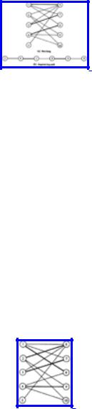
We can represent this situation by a graph as in Fig. 7.16 where the vertices are divided into two sets V1 and V2, such that vertices in the set V1 represent teachers and vertices in the set V2 courses. That teacher v is qualified to teach course w is represented by an edge (v, w). A graph such as this whose vertices can be divided into two disjoint groups with each edge having one end in each group is called bipartite. Assigning a teacher a course is equivalent to selecting an edge between a teacher vertex and a course vertex.

Fig. 7.16. A bipartite graph.

The matching problem can be formulated in general terms as follows. Given a graph G =(V, E), a subset of the edges in E with no two edges incident upon the same vertex in V is called a matching. The task of selecting a maximum subset of such edges is called the maximal matching problem. The heavy edges in Fig. 7.16 are an example of one maximal matching in that graph. A complete matching is a matching in which every vertex is an endpoint of some edge in the matching. Clearly, every complete matching is a maximal matching.

There is a straightforward way to find maximal matchings. We can systematically generate all matchings and then pick one that has the largest number of edges. The difficulty with this method is that it has a running time that is an exponential function of the number of edges.

There are more efficient algorithms for finding maximal matchings. These algorithms generally use a technique known as "augmenting paths." Let M be a matching in a graph G. A vertex v is matched if it is the endpoint of an edge in M. A path connecting two unmatched vertices in which alternate edges in the path are in M is called an augmenting path relative to M. Observe that an augmenting path must be of odd length, and must begin and end with edges not in M. Also observe that given an augmenting path P we can always find a bigger matching by removing from M those edges that are in P, and then adding to M the edges of P that were initially not in M. This new matching is M Å P where Å denotes "exclusive or" on sets. That is, the new matching consists of those edges that are in M or P, but not in both.

http://www.ourstillwaters.org/stillwaters/csteaching/DataStructuresAndAlgorithms/mf1207.htm (16 of 22) [1.7.2001 19:15:36]

Data Structures and Algorithms: CHAPTER 7: Undirected Graphs

Example 7.9. Figure 7.17(a) shows a graph and a matching M consisting of the heavy edges (1, 6), (3, 7), and (4, 8). The path 2, 6, 1, 8, 4, 9 in Fig. 7.17(b) is an augmenting path relative to M. Figure 7.18 shows the matching (l, 8), (2, 6), (3, 7), (4, 9) obtained by removing from M those edges that are in the path, and then adding to M the other edges in the path.

Fig. 7.17. A matching and an augmenting path.

The key observation is that M is a maximal matching if and only if there is no augmenting path relative to M. This observation is the basis of our maximal matching algorithm.

Suppose M and N are matchings with ½M½ < ½N½. (½M½ denotes the number of edges in M.) To see that M Å N contains an augmenting path relative to M consider the graph G' = (V, M Å N). Since M and N are both matchings, each vertex of V is an endpoint of at most one edge from M and an endpoint of at most one edge from N. Thus each connected component of G' forms a simple path (possibly a cycle) with edges alternating between M and N. Each path that is not a cycle is either an augmenting path relative to M or an augmenting path relative to N depending on whether it has more edges from N or

Fig. 7.18. The larger matching.

from M. Each cycle has an equal number of edges from M and N. Since ½M½ < ½N½, M Å N has more edges from N than M, and hence has at least one augmenting path relative to M.

We can now outline our procedure to find a maximal matching M for a graph G = (V, E).

http://www.ourstillwaters.org/stillwaters/csteaching/DataStructuresAndAlgorithms/mf1207.htm (17 of 22) [1.7.2001 19:15:36]