Data-Structures-And-Algorithms-Alfred-V-Aho

Data Structures and Algorithms: CHAPTER 8: Sorting

bubblesort in Fig. 8.1. No matter what recordtype is, swap takes a constant time. Thus lines (3) and (4) of Fig. 8.1 take at most c1 time units for some constant c1. Hence for a fixed value of i, the loop of lines (2- 4)

var

lowkey: keytype; { the currently smallest key found on a pass through A[i], . . . , A[n] }

lowindex : integer; { the position of lowkey } begin

(1)for i := 1 to n-1 do begin

{select the lowest among A[i], . . . , A[n] and swap it with

A[i] }

(2)lowindex := i;

(3)lowkey := A[i].key;

(4)for j := i + 1 to n do

{compare each key with current lowkey }

end;

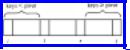
Fig. 8.7. Selection sort.

Fig. 8.8. Passes of selection sort.

takes at most c2(n-i) steps, for some constant c2; the latter constant is somewhat larger than c1 to account for decrementation and testing of j. Consequently, the entire program takes at most

steps, where the term c3n accounts for incrementating and testing i. As the latter

http://www.ourstillwaters.org/stillwaters/csteaching/DataStructuresAndAlgorithms/mf1208.htm (6 of 44) [1.7.2001 19:22:21]

Data Structures and Algorithms: CHAPTER 8: Sorting

formula does not exceed (c2/2+c3)n2, for n ³ 1, we see that the time complexity of

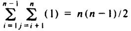
bubblesort is O(n2). The algorithm requires W(n2) steps, since even if no swaps are ever needed (i.e., the input happens to be already sorted), the test of line (3) is executed n(n - 1)/2 times.

Next consider the insertion sort of Fig. 8.5. The while-loop of lines (4-6) of Fig. 8.5 cannot take more than O(i) steps, since j is initialized to i at line (3), and decreases each time around the loop. The loop terminates by the time j = 1, since A[0] is -¥, which forces the test of line (4) to be false when j = 1. We may conclude

that the for-loop of lines (2-6) takes at most steps for some constant c. This sum is O(n2).

The reader may check that if the array is initially sorted in reverse order, then we actually go around the while-loop of lines (4-6) i-1 times, so line (4) is executed times. Therefore, insertion sort requires W(n2) time in the worst case. It can be shown that this smaller bound holds in the average case as well.

Finally, consider selection sort in Fig. 8.7. We may check that the inner for-loop of lines (4-7) takes O(n-i) time, since j ranges from i+1 to n. Thus the total time taken

by the algorithm is c , for some constant c. This sum, which is cn(n - 1)/2, is seen easily to be O(n2). Conversely, one can show that line (5), at least, is executed

times regardless of the initial array A, so selection sort takes W(n2) time in the worst case and the average case as well.

Counting Swaps

If the size of records is large, the procedure swap, which is the only place in the three algorithms where records are copied, will take far more time than any of the other steps, such as comparison of keys and calculations on array indices. Thus, while all three algorithms take time proportional to n2, we might be able to compare them in more detail if we count the uses of swap.

To begin, bubblesort executes the swap step of line (4) of Fig. 8.1 at most

http://www.ourstillwaters.org/stillwaters/csteaching/DataStructuresAndAlgorithms/mf1208.htm (7 of 44) [1.7.2001 19:22:21]

Data Structures and Algorithms: CHAPTER 8: Sorting

times, or about n2/2 times. But since the execution of line (4) depends on the outcome of the test of line (3), we might expect that the actual number of swaps will be considerably less than n2/2.

In fact, bubblesort swaps exactly half the time on the average, so the expected number of swaps if all initial sequences are equally likely is about n2/4. To see this, consider two initial lists of keys that are the reverse of one another, say L1 = k1, k2 , .

. . , kn and L2 = kn, kn - 1, . . . , k1. A swap is the only way ki and kj can cross each other if they are initially out of order. But ki and kj are out of order in exactly one of

L1 and L2. Thus the total number of swaps executed when bubblesort is applied to L1

and L2 is equal to the number of pairs of elements, that is, ( ) or n(n - 1)/2. Therefore the average number of swaps for L1 and L2 is n(n - 1)/4 or about n2/4. Since all possible orderings can be paired with their reversals, as L1 and L2 were, we see that the average number of swaps over all orderings will likewise be about n2/4.

The number of swaps made by insertion sort on the average is exactly what it is for bubblesort. The same argument applies; each pair of elements gets swapped either in a list L or its reverse, but never in both.

However, in the case that swap is an expensive operation we can easily see that selection sort is superior to either bubblesort or insertion sort. Line (8) in Fig. 8.7 is outside the inner loop of the selection sort algorithm, so it is executed exactly n - 1 times on any array of length n. Since line (8) has the only call to swap in selection sort, we see that the rate of growth in the number of swaps by selection sort, which is O(n), is less than the growth rates of the number of swaps by the other two algorithms, which is O(n2). Intuitively, unlike bubblesort or insertion sort, selection sort allows elements to "leap" over large numbers of other elements without being swapped with each of them individually.

A useful strategy to use when records are long and swaps are expensive is to maintain an array of pointers to the records, using whatever sorting algorithm one chooses. One can then swap pointers rather than records. Once the pointers to the records have been arranged into the proper order, the records themselves can be arranged into the final sorted order in O(n) time.

Limitations of the Simple Algorithms

We should not forget that each of the algorithms mentioned in this section has an O(n2) running time, in both the worst case and average case. Thus, for large n, none

http://www.ourstillwaters.org/stillwaters/csteaching/DataStructuresAndAlgorithms/mf1208.htm (8 of 44) [1.7.2001 19:22:21]

Data Structures and Algorithms: CHAPTER 8: Sorting

of these algorithms compares favorably with the O(nlogn) algorithms to be discussed in the next sections. The value of n at which these more complex O(nlogn) algorithms become better than the simple O(n2) algorithms depends on a variety of factors such as the quality of the object code generated by the compiler, the machine on which the programs are run, and the size of the records we must swap. Experimentation with a time profiler is a good way to determine the cutover point. A reasonable rule of thumb is that unless n is at least around one hundred, it is probably a waste of time to implement an algorithm more complicated than the simple ones discussed in this section. Shellsort, a generalization of bubblesort, is a simple, easy- to-implement O(n1.5) sorting algorithm that is reasonably efficient for modest values of n. Shellsort is presented in Exercise 8.3.

8.3 Quicksort

The first O(nlogn) algorithm† we shall discuss, and probably the most efficient for internal sorting, has been given the name "quicksort." The essence of quicksort is to sort an array A[1], . . . , A[n] by picking some key value v in the array as a pivot element around which to rearrange the elements in the array. We hope the pivot is near the median key value in the array, so that it is preceded by about half the keys and followed by about half. We permute the elements in the array so that for some j, all the records with keys less than v appear in A[1] , . . . , A[ j], and all those with keys v or greater appear in A[j+ 1], . . . , A[n]. We then apply quicksort recursively to A[1], . . . , A[j] and to A[j + 1] , . . . , A[n] to sort both these groups of elements. Since all keys in the first group precede all keys in the second group, the entire array will thus be sorted.

Example 8.4. In Fig. 8.9 we display the recursive steps that quicksort might take to sort the sequence of integers 3, 1, 4, 1, 5, 9, 2, 6, 5, 3. In each case, we have chosen to take as our value v the larger of the two leftmost distinct values. The recursion stops when we discover that the portion of the array we have to sort consists of identical keys. We have shown each level as consisting of two steps, one before partitioning each subarray, and the second after. The rearrangement of records that takes place during partitioning will be explained shortly.

Let us now begin the design of a recursive procedure quicksort(i, j) that operates on an array A with elements A[1] , . . . , A[n], defined externally to the procedure. quicksort(i, j) sorts A[i] through A[j], in place. A preliminary sketch of the procedure is shown in Fig. 8.10. Note that if A[i], . . . , A[ j] all have the same key, the procedure does nothing to A.

We begin by developing a function findpivot that implements the test of line (1) of

http://www.ourstillwaters.org/stillwaters/csteaching/DataStructuresAndAlgorithms/mf1208.htm (9 of 44) [1.7.2001 19:22:21]

Data Structures and Algorithms: CHAPTER 8: Sorting

Fig. 8.10, determining whether the keys of A[i], . . . , A[j] are all the same. If findpivot never finds two different keys, it returns 0. Otherwise, it returns the index of the larger of the first two different keys. This larger key becomes the pivot element. The function findpivot is written in Fig. 8.11.

Next, we implement line (3) of Fig. 8.10, where we face the problem of permuting A[i], . . . , A[j], in place‡, so that all the keys smaller than the pivot value appear to the left of the others. To do this task, we introduce two cursors, l and r, initially at the left and right ends of the portion of A being sorted, respectively. At all times, the elements to the left of l, that is, A[i], . . . , A[l - 1] will have keys less than the pivot. Elements to the right of r, that is, A[r+1], . . . , A[j], will have keys equal to or greater than the pivot, and elements in the middle will be mixed, as suggested in Fig. 8.12.

Initially, i = l and j = r so the above statement holds since nothing is to the left of l or to the right of r. We repeatedly do the following steps, which move l right and r left, until they finally cross, whereupon A[i], . . . , A[l - 1] will contain all the keys less than the pivot and A[r+1], . . . , A[j] all the keys equal to or greater than the pivot.

1.Scan. Move l right over any records with keys less than the pivot. Move r left over any keys greater than or equal to the pivot. Note that our

Fig. 8.9. The operation of quicksort.

selection of the pivot by findpivot guarantees that there is at least one key less than the pivot and at least one not less than the pivot, so l and r will surely come to rest before moving outside the range i to j.

2.Test. If l > r (which in practice means l = r+1), then we have successfully partitioned A[i], . . . , A[j], and we are done.

3.Switch. If l < r (note we cannot come to rest during the scan with l = r, because one or the other of these will move past any given key), then

(1) if A[i] through A[j] contains at least two distinct keys then begin

http://www.ourstillwaters.org/stillwaters/csteaching/DataStructuresAndAlgorithms/mf1208.htm (10 of 44) [1.7.2001 19:22:21]

Data Structures and Algorithms: CHAPTER 8: Sorting

(2)let v be the larger of the first two distinct keys found;

(3)permute A[i], . . . ,A[j] so that for some k between

i + 1 and j, A[i], . . . ,A[k - 1 ] all have keys less

than

v and A[k], . . . ,A[j] all have keys ³ v;

(4)quicksort(i, k - 1 );

(5)quicksort(k, j)

end

Fig. 8.10. Sketch of quicksort.

function findpivot ( i, j: integer ) :integer;

{ returns 0 if A[i], . . . ,A[j] have identical keys, otherwise returns the index of the larger of the leftmost two different keys } var

firstkey: keytype; { value of first key found, i.e., A[i].key } k: integer; { runs left to right looking for a different key }

begin

firstkey := A[i].key;

for k := i + 1 to j do {scan for different key}

if A[k].key > firstkey then { select larger key } return (k)

else if A[k].key < firstkey then return (i);

return (0) { different keys were never found } end; { findpivot }

Fig. 8.11. The procedure findpivot.

Fig. 8.12. Situation during the permutation process.

swap A[l] with A[r]. After doing so, A[l] has a key less than the pivot and A[r] has a key at least equal to the pivot, so we know that in the next scan phase, l will move at least one position right, over the old A[r], and r will move at least one position left.

The above loop is awkward, since the test that terminates it is in the middle. To put it in the form of a repeat-loop, we move the switch phase to the beginning. The

http://www.ourstillwaters.org/stillwaters/csteaching/DataStructuresAndAlgorithms/mf1208.htm (11 of 44) [1.7.2001 19:22:21]

Data Structures and Algorithms: CHAPTER 8: Sorting

effect is that initially, when i = l and j = r, we shall swap A[i] with A[j]. This could be right or wrong; it doesn't matter, as we assume no particular order for the keys among A[i], . . . , A[j] initially. The reader, however, should be aware of this "trick" and not be puzzled by it. The function partition, which performs the above operations and returns l, the point at which the upper half of the partitioned array begins, is shown in Fig. 8.13.

function partition ( i, j: integer; pivot: keytype ): integer; { partitions A[i], . . . ,A[j] so keys < pivot are at the left and keys ³ pivot are on the right. Returns the

beginning of the

group on the right. } var

l, r: integer; { cursors as described above } begin

(1)l := i;

(2)r := j; repeat

Fig. 8.13. The procedure partition.

We are now ready to elaborate the quicksort sketch of Fig. 8.10. The final program is shown in Fig. 8.14. To sort an array A of type array[1..n] of recordtype we simply call quicksort(1, n).

The Running Time of Quicksort

We shall show that quicksort takes O(nlogn) time on the average to sort n elements, and O(n2) time in the worst case. The first step in substantiating both claims is to prove that partition takes time proportional to the number of elements that it is called upon to separate, that is, O(j - i + 1) time.

http://www.ourstillwaters.org/stillwaters/csteaching/DataStructuresAndAlgorithms/mf1208.htm (12 of 44) [1.7.2001 19:22:21]

Data Structures and Algorithms: CHAPTER 8: Sorting

procedure quicksort ( i, j: integer );

{ sort elements A[i], . . . ,A[j] of external array A } var

pivot: keytype; { the pivot value }

pivotindex: integer; { the index of an element of A where key is the pivot }

k: integer; { beginning index for group of elements ³

pivot } begin

(1)pivotindex := findpivot(i, j);

(2)if pivotindex <> 0 then begin { do nothing if all keys are equal }

end

end; { quicksort }

Fig. 8.14. The procedure quicksort.

To see why that statement is true, we must use a trick that comes up frequently in analyzing algorithms; we must find certain "items" to which time may be "charged," and then show how to charge each step of the algorithm so no item is charged more than some constant. Then the total time spent is no greater than this constant times the number of "items."

In our case, the "items" are the elements from A[i] to A[j], and we charge to each element all the time spent by partition from the time l or r first points to that element to the time l or r leaves that element. First note that neither l nor r ever returns to an element. Because there is at least one element in the low group and one in the high group, and because partition stops as soon as l exceeds r, we know that each element will be charged at most once.

We move off an element in the loops of lines (4) and (6) of Fig. 8.13, either by increasing l or decreasing r. How long could it be between times when we execute l : = l + 1 or r := r - 1? The worst that can happen is at the beginning. Lines (1) and (2) initialize l and r. Then we might go around the loop without doing anything to l or r. On second and subsequent passes, the swap at line (3) guarantees that the whileloops of lines (4) and (6) will be successful at least once each, so the worst that can be charged to an execution of l := l + 1 or r := r - 1 is the cost of line (1), line (2),

http://www.ourstillwaters.org/stillwaters/csteaching/DataStructuresAndAlgorithms/mf1208.htm (13 of 44) [1.7.2001 19:22:21]

Data Structures and Algorithms: CHAPTER 8: Sorting

twice line (3), and the tests of lines (4), (6), (8), and (4) again. This is only a constant amount, independent of i or j, and subsequent executions of l := l + 1 or r := r - 1 are charged less -- at most one execution of lines (3) and (8) and once around the loops of lines (4) or (6).

There are also the final two unsuccessful tests at lines (4), (6), and (8), that may not be charged to any "item," but these represent only a constant amount and may be charged to any item. After all charges have been made, we still have some constant c so that no item has been charged more than c time units. Since there are j - i + 1 "items," that is, elements in the portion of the array to be sorted, the total time spent by partition(i, j, pivot) is O(j - i + 1).

Now let us turn to the running time spent by quicksort(i, j). We can easily check that the time spent by the call to findpivot at line (1) of Fig. 8.14 is O(j - i + 1), and in most cases much smaller. The test of line (2) takes a constant amount of time, as does step (3) if executed. We have just argued that line (4), the call to partition, will take O(j - i + 1) time. Thus, exclusive of recursive calls it makes to quicksort, each individual call of quicksort takes time at most proportional to the number of elements it is called upon to sort.

Put another way, the total time taken by quicksort is the sum over all elements of the number of times that element is part of the subarray on which a call to quicksort is made. Let us refer back to Fig. 8.9, where we see calls to quicksort organized into levels. Evidently, no element can be involved in two calls at the same level, so the time taken by quicksort can be expressed as the sum over all elements of the depth, or maximum level, at which that element is found. For example, the 1's in Fig. 8.9 are of depth 3 and the 6 of depth 5.

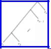
In the worst case, we could manage to select at each call to quicksort a worst possible pivot, say the largest of the key values in the subarray being sorted. Then we would divide the subarray into two smaller subarrays, one with a single element (the element with the pivot as key) and the other with everything else. That sequence of partitions leads to a tree like that of Fig. 8.15, where r1, r2 , . . . , rn is the sequence of records in order of increasing keys.

Fig. 8.15. A worst possible sequence of pivot selections.

http://www.ourstillwaters.org/stillwaters/csteaching/DataStructuresAndAlgorithms/mf1208.htm (14 of 44) [1.7.2001 19:22:21]

Data Structures and Algorithms: CHAPTER 8: Sorting

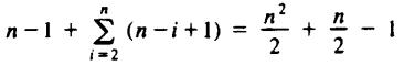
The depth of ri is n - i + 1 for 2 ≤ i ≤ n, and the depth of r1 is n - 1. Thus the sum of the depths is

which is Ω(n2). Thus in the worst case, quicksort takes time proportional to n2 to sort n elements.

Average Case Analysis of Quicksort

Let us, as always, interpret "average case" for a sorting algorithm to mean the average over all possible initial orderings, equal probability being attributed to each possible ordering. For simplicity, we shall assume no two elements have equal keys. In general, equalities among elements make our sorting task easier, not harder, anyway.

A second assumption that makes our analysis of quicksort easier is that, when we call quicksort(i, j), then all orders for A [i], . . . , A [j] are equally likely. The justification is that prior to this call, no pivots with which A [i], . . . , A [j] were compared distinguished among them; that is, for each such pivot v, either all were less than v or all were equal to or greater than v. A careful examination of the quicksort program we developed shows that each pivot element is likely to wind up near the right end of the subarray of elements equal to or greater than this pivot, but for large subarrays, the fact that the minimum element (the previous pivot, that is) is likely to appear near the right end doesn't make a measurable difference.†

Now, let T(n) be the average time taken by quicksort to sort n elements. Clearly T(1) is some constant c1, since on one element, quicksort makes no recursive calls to itself. When n > 1, since we assume all elements have unequal keys, we know quicksort will pick a pivot and split the subarray, taking c2n time to do this, for some constant c2, then call quicksort on the two subarrays. It would be nice if we could

claim that the pivot was equally likely to be any of the first, second, . . . , nth element in the sorted order for the subarray being sorted. However, to guarantee ourselves that quicksort would find at least one key less than each pivot and at least one equal to or greater than the pivot (so each piece would be smaller than the whole, and therefore infinite loops would not be possible), we always picked the larger of the first two elements found. It turns out that this selection doesn't affect the distribution of sizes of the subarrays, but it does tend to make the left groups (those less than the

http://www.ourstillwaters.org/stillwaters/csteaching/DataStructuresAndAlgorithms/mf1208.htm (15 of 44) [1.7.2001 19:22:21]