

10789
.pdfSilaeva A. M.
Nizhny Novgorod State University of Architecture and Civil Engineering
THE PROBLEMS OF MODERN INDUSTRIAL ARCHITECTURE
The industrial architecture is the architecture of factories, all kinds of hydraulic structures (for example, bridges and hydraulic stations), the entire system of heat power engineering and other industrial buildings.
Think about typical Russian industrial building. Usually it looks like some big grey box, with which the most positive person can be bored.
The aim of industrial architecture is to provide convenient conditions for company’s workers; or, in short, help people love their working process.
There are two ways to attain a necessary effect: when architect is proecting a building he means to consider two main options – shape and color scheme. Speaking of Russian situation because of features of climate in our country is the lack of sun, lower temperature – looks like we should paying attention on color design more then on shapes.
The architecture is a thing that controls the process of environment organization; how the world will be looks like tomorrow depends on our today’s decisions, and what do we have? There are a lot of shapeless boxes, with rare exceptions.
Unlike Russian entrepreneurs, their western colleagues pay more attention to industrial architecture. There is even one of the branch of tourism is the industrial one. And it’s not only a popular entertainment but also it helps the entrepreneurs to attract people’s attention to the brand.
These days, factories aren't perceived as the drivers of sociological evolution and architects aren't caught up in debate of industrial typologies, yet there's been a wide range of approaches to these buildings still percolating in the background. Some of these buildings look futuristic and Daft Punk-y, other could be straight out of an Andreas Gursky photograph. What will the architecture of industry look like in the future?
For example, in our country we have a few great projects – one of them is
Chelyabinsk Tube Rolling Plant’s departmens which was included at the all of lists the most beautiful industrial buildings. Also there are the first objects of innovation center “Skolkovo” which have to be mentioned.
Unfortunately, there are not so many |
projects like those ones in Russia. |
|||||
However, we can estimate the decisions |
some industrial |
territories |
– for |
|||
example, |
Technopark |
in |
Akademgorodok, Novosibirsk. |
And |
||
a town in Verkhneuslonsky |
District of the Republic of |
Tatarstan, Russia, |
||||
a satellite of Kazan, the capital of the republic. |
|
|
||||
450
Summarizing the discussion above, there are couple things to say: at first, the impressed industrial architecture exists. It’s developing, the new materials and technological decisions appear.
And, the second thing, we should change our attitude about industrial architecture from indifferent to interested. It has many positive consequences – the right architecture decisions may rise up working efficiently, the industrial tourism helps to take benefit.
Our country already has an experience on to design attractive industrial architectural objects, so we should just keep going on.
Turtsev M.A., Aleshugina E.A.
Nizhny Novgorod State University of Architecture and Civil Engineering
METHODS OF FINDING THE MINIMUM OF FUNCTION OF SEVERAL VARUABLES: METHOD OF GRADIENT PROJECTION IN CASE OF LINEAR CONSTRAINTS
In his activities the person has to meet either explicitly or implicitly with optimization. This is due to what challenges confront the person, and how it is complicated. Problem to be solved, for example, in economics, in planning, in management, in the design of industrial facilities require the ownership of a particular mathematical apparatus, allowing to search for the best variant from the point of view of the target. With all the variety of optimization problems to give general methods for their solution can only be mathematics, dramatic expansion of the application of which is associated with the advent of computers, which led to the mathematization not only physics but also chemistry, biology, economics, psychology, medicine — almost all sciences. The essence of mathematization is to construct mathematical models of processes and phenomena and to develop methods of their study.
The use of mathematical tools in the solution of optimization problems involves the formulation of the problem of interest in the language of mathematics, giving quantitative estimates of the possible options is "better", "worse".
Many optimization problems boil down to finding the smallest or largest values of some function, which is called the objective function. In this case, research methods significantly depend on the properties of the objective function and the information about it that may be available to solve the problem and its solution.
The most simple from a mathematical point of view, the cases when the objective function is a differentiable function. In this case, to study its properties, areas of increasing and decreasing, points of local extreme can be used derivative. In the last decades in terms of scientific and technological
451

progress, the range of optimization problems posed by the practice has expanded significantly. In many of them the objective function value can be the result of numerical calculations or taken from experiment. Such tasks are more complex in their decision not to investigate an objective function using the derivative. This led to the development of special methods, designed for a wide use of computers. It should also be borne in mind that the complexity of the problem significantly depends on the dimension of the target function, i.e. the number of its arguments.
Step-by-step algorithm of the method of gradient projection (in the case of linear constraints):
Step 1: If the initial value belongs to the limits, displaying a message that the starting point is outside the borders, and stop. Otherwise proceed to step 2.
Step 2: Remember the coordinates of the point. Go to step 3. Step 3: Gradient of the function is calculated.
Step 4: The projection of the gradient is calculated, according to the algorithm of the method of finding the projection of the gradient.
Step 5: Check the condition: if the projection of the point on the axes is not equal to 0 then go to step 6, otherwise stop and output the result.
Step 6: Step is calculated along the projection of the gradient shag. Step 7: The calculated step according to the method of the Golden section
in the interval from 0 to shag.
Step 8: The following approximation is computed with the step, computed by the method of Golden section.
Step 9: Check the stopping criterion: if , then
stop and output the result. Otherwise proceed to step 2.
Method of finding the projection of the gradient:
There are 3 cases when you need to find the projection of the gradient vector:
First case: the projection of the gradient of  equal to antigradient function
  in case when
 .
.
Second case: the projection of the gradient of  equal to the maximum of
  in case when
  equal to its left boundary of the constraint c.
Third case: the projection of the gradient of  is the minimum of
  in case
  equal to its right boundary of the constraint d.
Method of finding step (in the case of linear constraints along the projection of the gradient of the function):
If the projection of the gradient of  is not 0, then: Looking for step 1 according to the formula:
Looking for step 2 according to the formula:
452

The desired step shag is the minimum of  и
и  .
.
The point B(0;0) is a point of local minimum of the function, calculated with analytical method.
The graph of the function [Graph 1]:
Graph 1. The graph of the function
Table 1. The results of software calculations with different precisions and initial points
№ |
Point : |
Precision |
The |
The extreme |
Deviation |
|
|
|
|
|
number of |
point |
from |
equal |
|
|
|
|
iterations N |
|
point |
|
|
|
|
|
|
|
X- |
|
|
|
|
|
|
|
|
|
|
1 |
(5; 5) |
0.0001 |
2 |
(1; 1) |
(0.0; 0.0) |
|
|
|
|
|
|
|
|
|
|
2 |
(9; 9) |
0.001 |
10 |
(1; 1) |
(0.0; |
|
|
|
|
|
|
|
0.0) |
|
|
|
|
|
|
|
|
|
|
3 |
(4; 7) |
0.02 |
5 |
(0,998753; |
(0.001247; |
|
|
|
|
|
|
1,00034) |
0.00034) |
|
|
|
|
|
|
|
|
|
|
4 |
(0; 4) |
0.001 |
5 |
(0.99181; |
(0.00819; |
|
|
|
|
|
|
0,994283) |
0.005717) |
|
|
|
|
|
|
|
|
|
|
5 |
(0; 1) |
0.000001 |
3 |
(1; 1) |
(0.0; 0.0) |
|
|
|
|
|
|
|
|
|
|
6 |
(4; 9) |
0.001 |
11 |
(0.999383; |
(0.000617; |
- |
|
|
|
|
|
1.00283) |
0,00283) |
|
|
|
|
|
|
|
|
|
|
7 |
(8; 8) |
0.001 |
5 |
(0.999999; |
(0.000001; |
|
|
|
|
|
|
0.999999) |
0.000001) |
|
|
|
|
|
|
|
|
|
|
453
In conclusion, it is necessary to say that gradient methods converge to a minimum with a high rate (exponentially) for smooth convex functions.
However, in practice, as a rule, the minimized functions have the illconditioned Hessian matrix. The values of such functions along certain lines change much faster (not rarely by several orders of magnitude) than in other directions. The surface level in the simplest case of strongly drawn, and in more complex cases, curve and represent the ravines. Functions with such properties is called ravine. The direction of antigradient these functions significantly deviates from the direction to the minimum point, which leads to slow speed of convergence.
The convergence rate of gradient methods significantly depends on how accurately the computed gradient. Loss of precision and it usually occurs in the vicinity of low points or gully situation, may break the convergence of the gradient descent process. Due to these reasons, gradient methods are often used in combination with other more effective methods at the initial stage of solving the problem. In this case, the point  is far from the valleys and steps in the direction of antigradient allow to achieve a significant decreasing functions.
References
1.Optimization techniques : proc.manual for schools / V. A. Goncharov.
—M.: Publishing house of yurayt ; ID yurait, 2014. — 191 p. — Series : the Bachelor. Basic course.
2.M. Bazara, K. Shetty. Nonlinear programming. Theory and algorithms: TRANS. from English. – M.:Mir,1982.583 p.
Sobolev V.A., Aleshugina E.A.
Nizhny Novgorod State University of Architecture and Civil Engineering
NONLINEAR PROGRAMMING
In most engineering problems, the construction of a mathematical model cannot be reduced to the problem of linear programming.
Mathematical models in the problems of designing objects or technological processes must reflect the actual physical and, usually, nonlinear processes occurring in them.
As a result, most of mathematical programming problems, that occur in research projects and in design tasks are problems of non-linear programming.
The purpose of this work is to consider the Hooke-Jeeves method with the step search by the bitwise approximation method, to examine the basic concepts, formulas, theorems encountered in solving problems, to consider the basic
454
methods of solving extremum and optimization problems with implementation in one of the programming languages.
Formulation of the problem:
The tasks of this work include the following items:
Studying the Hooke-Jeeves method to find an unconditional local
extremum of a function F(x) = 194*(x1^2)+376*x1*x2+194*(x2^2)+31*x1229*x2+4.
Studying the bitwise approximation method to find the step.
Solving the problem of non-linear programming using the methods above.
Implementation of these methods using one of the programming languages
The method of solving the problem:
The Hooke-Jeeves method is used to find an unconditional local extremum of a function and refers to direct methods. It means that it is based directly on the values of the function. This method was developed in 1961, but it is still one of the most effective. The search is divided into two stages: exploring search and pattern search where the two previous points are used.
Bitwise approximation method is an improvement of the method of enumeration. The search of a minimum point of the function is carried out with a variable step. In the beginning, the step is assumed to be sufficiently large and the segment containing the minimum point is approximately found out. Then, with a higher accuracy, the required minimum point is found on this segment.
Algorithm of the methods:
1) Hooke-Jeeves method
Step 1. Exploring search. Set X0i>0, find h by the bitwise approximation method, calculate X1i= X0i+h*di
Step 2. Pattern search. Find h by the bitwise approximation method. Calculate X2=X1+h*(X1-X0) using X0 and X1.
Step 3. Set precision e>0. If |F(X2)-F(X1)|<e, then stop, X*=X2,
Fmin=F(X2). Else X0=X2, go to step 1.
2) Bitwise approximation method.
Step 1. Set segment [a; b] and divide it into 4 parts: h=(b-a)/4.
Step 2. Set precision e>0. If h<e, then stop, x*=(b+a)/2. Else xi+1=xi+h;
f(xi); f(xi+1).
Step 3. If f(xi+1)< f(xi) then go to step 2. Else b= xi+1 hnew, =h/4.
Step 4. If hnew<e, then stop, x*=(b+a)/2. Else xi+1=xi-h; f(xi); f(xi+1); go to step 3.
Calculation results [Table 1]:
F(x) = 194*(x1^2)+376*x1*x2+194*(x2^2)+31*x1-229*x2+4 [Fig. 1.]
455

Fig 1. Function graph
Exact value - X*= (-10.7287 ; 10.9922); F(X*) = -1417.15
|
|
|
Table 1. Calculation results |
||
Initial value |
Precision e |
Number |
Extremum value |
Observational |
|
x |
|
of |
|
error |
|
|
|
iterations |
|
|
|
|
|
|
X*=(-10.7287 ; |
-0% |
|
-11; 11 |
0.01 |
1 |
10.9922); F(X*) = - |
|
|
|
|
||||
|
|
|
1417.15 |
|
|
|
|
|
X*=(-11.6215 ; |
|
|
-12; 12 |
0.01 |
2 |
11.8570); F(X*) = - |
-0.7% |
|
|
|
|
1407.21 |
|
|
|
|
|
X*=(-10.8308 ; |
0.0016% |
|
-12; 12 |
0.001 |
11 |
11,1029); F(X*) = - |
|
|
|
|
||||
|
|
|
1416.92 |
|
|
Search trajectory [Fig. 2]: |
|
|
|
||
|
|
|
Table 2. Initial value and precision |
||
Initial value X0 |
|
(-12 ; 12) |
|
|
|
Precision e |
|
0.01 |
|
|
|
456
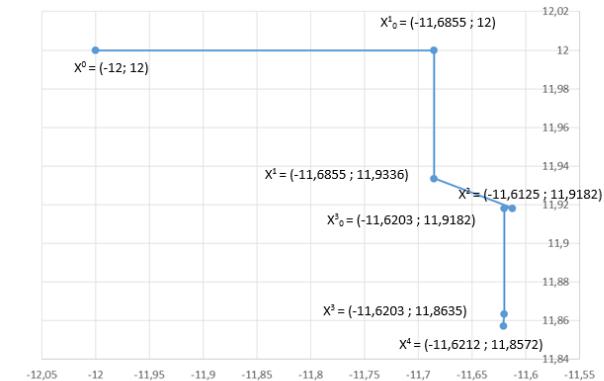
Fig. 2. Search trajectory
In the course of this work the Hooke-Jeeves method was studied which is considered one of the most effective methods of searching for an unconditional local extremum of a function.
The method of bitwise approximation was also considered. The work is served to find the step in the Hooke-Jeeves method.
Based on the results of program and analytical calculations, it can be concluded that the Hooke-Jeeves method is effective.
The value of the extremum found programmatically can differ from the value found analytically by 0.7% which may indicate a sufficient accuracy of the method.
Martemianova A.A., Aleshugina E.A.
Nizhny Novgorod State University of Architecture and Civil Engineering
OPTIMIZATION TECHNIQUES
We meet with optimization in any sphere of human activity both on a purely personal, and at the national level. Economic planning,management, design of complex objects is always aimed at finding the best option from the point of view of the intended goal.
457
For all the variety of optimization problems only mathematics can offer general methods of solving them, the sharp expansion of applications is connected with the appearance of a computer, which led to the mathematization not only of physics, but also of chemistry, biology, economics, psychology, medicine-practically all sciences. The essence of mathematization consists in constructing mathematical models of processes and phenomena and in developing methods for their investigation.
The use of a mathematical apparatus in solving optimization problems involves the formulation of a problem of interest in the language of mathematics, making quantitative estimates of possible variants in place of the words "better", "worse".
Many optimization problems are reduced to finding the smallest or largest value of some function, which is called the objective function. Such a formulation of the problem will be usual in the sequel. In this case, the research methods essentially depend on the properties of the objective function and that information about it, which can be considered accessible before the solution of the problem and in the solution process.
The simplest cases from a mathematical point of view are when the objective function is a differentiable function. In this case, a derivative can be used to study its properties (areas of increase and decrease, points of local extremum). In recent decades, under the conditions of scientific and technological progress, the range of optimization tasks set by practice has significantly expanded. In many of them, the values of the objective function can be obtained as a result of numerical calculations or taken from an experiment. Such problems are more complicated, in solving them one cannot study the objective function with the help of a derivative. This led to the development of special methods designed for the widespread use of computers. It should also be borne in mind that the complexity of the solution of the problem depends essentially on the dimension of the objective function, of the number of its arguments.
The purpose of my work is to study the method of steepest descent (the calculation of a one-dimensional function for finding the step by the parabolic approximation method).
The method of steepest descent.
The method of steepest descent is a variant of gradient descent. Here it is also assumed that pk = - f (xk), but the step size α_k from x(k + 1) = xk + α_k p ^
k, k = 0,1, ... is the result of the solution one-dimensional optimization
problems:
F_k (α) → min, F_k (α) = f (xk-α f (xk)), α> 0
that is, at each iteration in the antigradient direction - f (xk), an exhaustive descent is performed.
Method algorithm:
Step 1. Set the parameter ε> 0, select xεE_n. Compute f (x). Go to step 2.
458
Step 2. Calculate f (x) and check the condition for accuracy: | (| f (x) |) |
<ε. If it is satisfied, complete the calculations by putting x* = x, f * = f (x).
Otherwise go to step 3.
Step 3. Solve the problem of one-dimensional optimization F_k (α) → min, F_k (α) = f (xk-α f (xk)), α> 0
for xk = x, that is, find α*. Put x = x-α* f (x) and go to step 2. Method of parabolic approximation
Description of the method
The search for a minimum point by the methods of segment exclusion is based on a comparison of the values of the function at two points. With this comparison, the differences in the values of f (x) at these points are not taken into account, only their signs are important.
To take into account the information contained in relative changes in the values of f (x) at test points, polynomial approximation methods, whose main idea is that an approximating polynomial is constructed for the function f (x), and its minimum point serves as an approximation to x*. To effectively use these methods on the function f (x), an additional requirement is imposed for sufficient smoothness (at least, continuity).
The advantage of the method is the high rate of convergence.
To increase the accuracy of the approximation, one can, first, increase the order of the polynomial and, secondly, reduce the length of the approximation segment. The first way leads to a rapid complication of computational procedures, therefore in practice approximating polynomials of no higher than third order are used. At the same time, the reduction of the segment containing the minimum point of the unimodal function is not particularly difficult.
In the simplest method of polynomial approximation, the method of parabolas uses second-order polynomials. At each iteration of this method, a square trinomial is constructed whose graph (parabola) passes through three selected points of the graph of the function f (x)
Algorithm of the method of parabolic approximation. Algorithm of interval search.
Step 1: Take 2 points x1 and x3. We define them by searching for the interval [a; b]
Look for the right border (b)
1.Set the value of h and x0. We compute the function f (x0)
2.x1 = x0 + h
3.We assume that f (x1)
4.Compare the values: if f (x1)> f (x0), then b = hH, if not, then we consider the new step hH = 2 * h and go to step 2
5.We assume that as long as f (xn)> f (xn-1)
The left boundary (a) is searched in the same way, only the initial step (h) is taken with the opposite sign.
We obtain: a = x1
459