Chapter 10

MODELLING DRUG EFFECT USING

FRACTIONAL CALCULUS

Clara M. Ionescu*

Ghent University, Department of Electrical Energy,

Systems and Automation, Zwijnaarde, Belgium

Abstract

Closed loop control of depth of anesthesia (DOA) implies a good knowledge of the patient pharmaco-kinetics and -dynamics, i.e., the availability of a reliable model of the patient. This is necessary since prediction of drug effect in the body is essentially the main component of regulating DOA. Hitherto, this is done in a complex clinical environment, involving the anesthesiologist as a main decision-maker element. Obviously, the decision of administrating hypnotic and opioid drugs is a difficult one, since overand under-dosing are a peril for patient’s wellbeing and recovery. The expertise of the anesthesiologist and human factor make this decision a subjective one and may be difficult to justify in a mathematical framework. This chapter introduces emerging tools available on the 'engineering market' imported from the area of fractional calculus. Drug diffusion compartmental models are introduced and a novel interpretation of the classical drug-effect curve given. By employing tools from fractional calculus, model nonlinearity is avoided, allowing linear control strategies for automatic control of DOA systems.

Keywords: Analgesia, nonlinear dynamics, closed loop anesthesia, multivariable control, depth of anesthesia, drug effect interaction, fractional order impedance

Introduction

The emerging concepts of fractional calculus (FC) in biology and medicine have shown a great deal of success, explaining complex phenomena with a startling simplicity (Magin, 2006; Ionescu, 2013). It is clear that a major contribution of the concept of FC has been and remains still in the field of biology and medicine (West, 1990; Machado et al., 2013).

* Corresponding Author address: Email: claramihaela.ionescu@ugent.be.

Complimentary Contributor Copy

Fractional calculus generously allows integrals and derivatives to have any order, hence the generalization of the term fractional-order to that of general-order. Of all applications in biology, diffusion is the one most appealing from modeling point of view, since it allows characterizing a relatively complex process with parsimonious models.

Modeling drug dynamics in the body using compartmental models is perhaps one of the most popular modeling approaches (Jacques, 1985). These models are based on mathematical characterization of molecular biochemistry and transport phenomena in the body (Macheas & Iliadis, 2006). As such, diffusion plays an important role in drug assimilation, transport and clearance, and it is a physiological process, which can be well described by means of fractional calculus (Trujillo, 2006).

In this chapter, a fresh view upon the models for drug release and their effect will be given in the application of depth of anesthesia regulation. Although in this chapter only hypnosis will be discussed, general anesthesia consists of three components acting simultaneously on the patient’s vital signals, leading to an overall state of a) hypnosis b) neuromuscular blockade and c) analgesia (i.e., pain relief level).

Hypnosis is a general term indicating unconsciousness and the level of hypnosis is related to the infusion of hypnotic drug. Hypnosis is relatively well characterized and sensors to measure it by means of electroencephalogram (EEG) data are currently employed in standard clinical practice (Liu et al., 2011; Struys et al. 1998) and have been proven useful in closedloop control of anesthesia (Ionescu et al. 2008; Ionescu et al. 2011).

Neuromuscular blockade ensures that the patient remains paralyzed during surgical procedures and is also a relatively well-characterized process with standard sensors available (EMG-electromyography) (Ozcan et al., 2012). Analgesia represents the loss of pain sensation that results from a interruption in the nervous system pathway between the sense organ and the brain. Finally, sedation refers to a combined effect of hypnosis and analgesia (Kress et al., 2002). From the point of view of detection and measurement, analgesia is the sole component remaining to be de-mystified.

Figure 1. A personal view upon the high interdisciplinarity required to obtain a comprehensive picture of the anesthesia paradigm.

Complimentary Contributor Copy

If one would like to have optimal drug infusion rates into a patient with avoiding overand under-dosing, then accurate patient models are necessary (although not sufficient, since a good control methodology is also required) (Absalom et al., 2011). Accurate models may hold a realistic dynamic perspective for average populations datasets, but they are by far suboptimal when patient-individualized control is envisaged. This is due to the fact that interpatient variability has a strong impact on the perception and effectiveness of the drug into the body of the patient (i.e., drug effect, patient sensitivity to the drug, etc.). A schematic representation of the anesthesia paradigm in terms of its components is given in Figure 1. The hypnosis and neuromuscular blockade are well characterized, yet the analgesia component remains challenging for control purposes because no direct output measure is available. Hence, no specific models are yet available for analgesia effect in the human body during general anesthesia (i.e., unconsciousness).

Figure 2. An overview of inputs and outputs in the complex dynamic system of the human body during surgery and general anesthesia.

The absence of more objective measures and decision-making elements in the DOA regulating system is justified by the lack of direct measures of hypnosis and analgesia, as depicted in Figure 2. Hypnosis is a state of (un)consciousness and this is currently measured via an indirect measure, the electroencephalogram. Analgesia is a state of insensibility to pain stimuli (mechanical, thermal, etc.) and is measured via indirect measures such as facial stress, reaction to speech, reaction to electrical stimulation in the hand of the patient, etc. Clearly, of these two components, analgesia is the most subjective measurement. Efforts are being made to develop new sensor techniques and new horizons are explored for modeling this intricate process and to provide mathematical models to replace these subjective evaluations.

The pharmacokinetic (PK) models available in the literature are linear in terms of model parameters and dynamics (Schnider et al, 1998; 1999). Their frequency response is quasiidentical, less for a scaling factor in the gain (this accounts in part for the sensitivity to the drug with respect to the body mass index of the patient). The pharmacodynamic (PD) models are usually represented by nonlinear Sigmoid (Hill) curves and represent the relationship of the drug concentration to the drug effect in each patient. From patient-individualized control

Complimentary Contributor Copy

point of view, PD models are the most challenging part of the patient model andpose most challenges for control (i.e., highly nonlinear characteristic).

Fractional calculus offers tools to model such nonlinear characteristics as those of the PD models with less degree of nonlinearity in model parameters (Ionescu, 2013). The original purpose of this chapter is to put forward a fresh view to these models and to suggest how they can be integrated in the control paradigm of depth of anesthesia regulation.

The chapter is structured as follows: next, a brief introduction on the fractional calculus tools for modeling drug release and its effect is given. Section III depicts the classical methodology for PK-PD models in anesthesia and section IV presents the proposed PD modeling approach and some simulation results. Current limitations for the use of these models in a closed loop control paradigm are given and a conclusion section summarizes the main outcome of this paper.

Methods

Emerging Tools in the Field of Bio-Engineering

Pure empirical models such as input - output models are rather descriptive with loss of physiological insight into the drug absorption, transport, diffusion and release. However, from control point of view they are the most simple to obtain and to deliver information to the controller for deciding the optimal drug infusion rate necessary for the specific patient whose model is available. On the other hand, physiologically and bio-chemically based models are difficult to attain due to the extraordinary complexity of this process. For instance, the pathway of pain signaling into the body is depicted in Figure 3. It can be observed the various flows and complex bio-chemical reactions necessary to be modeled.

Figure 3. A diagram of the pathways of pain signaling in the human body.

In general, pain is a complicated process that involves an intricate interaction between a number of important chemicals found naturally in the brain and spinal cord. These chemicals,

Complimentary Contributor Copy

called neurotransmitters, transmit nerve impulses from one cell to another. The complex process of pain awareness can be divided in three main phases: (i) transduction, (ii) transmission and (iii) perception. The first phase, transduction, begins when a painful or noxious stimulus causes tissue damage. The damaged cells release substances that lead to the generation of an electric action potential. In the next phase (i.e., transmission of the pain signal) the electric action potential continues from the site of damage to the spinal cord, where it ascends up the spinal cord to higher centers in the brain. The third phase, perception, is the conscious awareness of pain. Treatment of pain-related suffering requires knowledge of how pain signals are initially interpreted and subsequently transmitted and perpetuated. Therefore, it is mandatory to first understand how an analgesic drug diffuses into the human body and how we can build models of pain signaling and transmission.

An intermediate solution is perhaps the use of semi-empirical models. Such a fairly simple model to employ in characterizing drug release is the power-law model:

where Mt and M∞ are cumulative amounts of drug released at time t and infinite time, respectively; and k is a constant reflecting the structural and geometrical characteristics of the system, and n is the release exponent (Higuchi, 1961). For purely diffusion-controlled release, n=0.5, while other values of n may be indicative of various diffusion conditions. These features of this model are of special interest in our study since we would like to look at the inter-patient variability from this standpoint.

Following the fundamental law of physics which applies to well stirred, homogeneous systems, it follows that the mean square displacement of the walker, <x2> in the random walk model is proportional to time (Kopelman, 1988; Rinaki et al., 2003):

However, in disordered systems, such as most biological environments, this is no longer proportional with time, but with the fractal walk dimension of the walker:

with Dw≠ 2. This property implies that scaling laws such as power laws are associated with kinetics of various processes taking place in the (biological) environment (i.e., tissue). Most biological tissues can be approximated in their properties by polymers. As such, the spatiotemporal porosity of a dynamically changing polymer is close to the percolation threshold for non-classical diffusion effects impinging on release kinetics.

Fractional calculus has shown in several (non)biological applications that classical diffusion as well as non-classical diffusion can be characterized by fractional order differintegrals models (Machado et al, 2013; Trujillo, 2006). It is possible to derive further the model from (1) in its Laplace equivalent, as indicated in (Magin, 2006). This result has regained the attention of the research community and current efforts are being directed

Complimentary Contributor Copy

towards providing pharmacokinetic models with fractional order differ-integrals (Dokoumetzidis and Macheras, 2009; Kytariolos et al, 2010; Dokoumetzidis et al., 2010; Popovic et al., 2011; Hennion and Hanert, 2013; Popovic et al, 2013; Copot et al., 2013; Ionescu et al., 2013), and their equivalent Laplace models of non-integer order, coined in the literature as FOIMs (fractional order impedance models) (Ionescu, 2013).

Classical PK-PD Models for Drug Diffusion

In order to control the depth of sedation based on predictive control strategies, a model capturing the dynamics of the patient is required. The selection of the model’s input and output variables is crucial for optimal control. Propofol is a commonly used hypnotic drug to induce general anesthesia (Absalom et al., 2011; Bailey & Haddad, 2005) and is also used to avoid awareness of pain. Sometimes is used together with Remifentanil, a strong opioid, to emphasize analgesia (i.e., pain relief). The two drugs have a synergic effect, obeying exactly the same behavior as that discussed in this section. For sake of simplicity, only the effects of one drug (i.e., Propofol) will be considered hereafter.

Using the electroencephalogram (EEG), several derived, computerized parameters like the BIS have been tested and validated as a promising measure of the hypnotic component of anesthesia. BIS values lie in the range of 0-100; whereas 90-100 range represents fully awake patients; 60-70 range and 40-60 range indicate light and moderate hypnotic state, respectively (Struys et al., 2003).

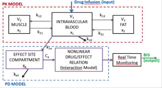
PK-PD blocks denote compartmental models. The PK-PD models most commonly used for propofol and remifentanil are the 4th order compartmental model described by Schnider et al., (1998, 1999) and they have the structure depicted in Figure 4:

Figure 4. General compartmental model of the patient, where PK denotes the pharmacokinetic model and PD denotes the pharmacodynamic model of an infused drug.

Complimentary Contributor Copy

In this figure x1 [mg] denotes the amount of drug in the central compartment. The blood concentration is expressed by x1/V1. The peripheral compartments 2 and 3 model the drug exchange of the blood with well and poorly diffused body tissues. The masses of drug in fast and slow equilibrating peripheral compartments are denoted by x2 and x3, respectively. The parameters kji, for i≠j, denote the drug transfer frequency from the jth to the ith compartment and u(t) [mg/s] is the infusion rate of the anesthetic drug into the central compartment. An additional hypothetical effect compartment was proposed to represent the lag between drug plasma concentration and drug response. The parameters kij of the PK models depend on age, weight, height and gender and the relations can be found in (Schnider 1998; 1999). The PKPD model is represented by the following equations:

The effect compartment receives drug from the central compartment by a first-order process and it is regarded as a volumeless additional compartment. Therefore, the drug transfer frequency from the central compartment to the effect-site compartment is equal to the frequency of drug removal from the effect-site compartment: ke0=k1e=0.456 [min-1] (Struys et al. 2003). Drug concentration in the effect site compartment is denoted by the variable Ce. The parameters kij of the PK models depend on age, weight, height and gender and can be calculated for Propofol:

where Cl1 is the rate at which the drug is cleared from the body, and Cl2 and Cl3 are the rates at which the drug is removed from the central compartment to the other two compartments by

The relation between the effect site concentration Ce and the BIS is given by a nonlinear sigmoid Hill curve:

Complimentary Contributor Copy

where E0 is the BIS value when the patient is awake; Emax is the maximum effect that can be achieved by the infusion of Propofol; C50 is the Propofol concentration at half of the

maximum effect and γ is a parameter which together with the C50 determines the patient sensitivity to the drug. Usually, E0 and Emax are usually considered equal to 100.

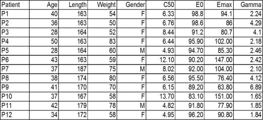
As explained earlier, the main challenge for control standpoint is the nonlinearity of the Hill curve given by (5) and the inherent inter-patient variability. To illustrate this to the reader, a realistic set of typical and atypical patients has been used, with the parameter values given in Table 1. The resulted Hill curves by simulating the PKPD model of these patients is shown in Figure 5.

Figure 5. Example of Hill curves from various patients illustrating the high-degree of interpatient variability.

For instance, Patient 3 and patient 9 require the same amount of effect site concentration before they start to react, but they have significantly different sensitivity to the drug effect. On the other hand, patient 6 requires less effect site concentrations to initiate the reaction in BIS, but the response is very slow. Moreover, it can be generalized that below a certain threshold value for the effect site concentration, the BIS(t) does not vary significantly. Such a threshold interval is used in practice to apply target-controlled infusion, which is in fact an open loop control policy. This specific intial strategy provides a desired effect site concentration in the patient, but does not take into account the actual measured BIS. Obviously, this is only useful in the induction phase of anesthesia, i.e., until a certain ΔBIS is achieved.

Complimentary Contributor Copy

Table 1. Characteristic variables for each of the virtual realistic 12 patients used in this study as from (Ionescu et al, 2008)

It is obvious that all these differences in reactions from patients to the same amount of drug infused in their body require a high degree of robustness from the controller. The drawback is a conservative control, which may not always deliver the expected performance, e.g., when disturbances need to be removed fast to avoid awareness in the patient.

Consequently, a significant strain is put on the controller’s task to keep the closed loop performance within the same specifications for all types of patients.

Hybrid Models emerging from Classical PK-PD and FOIMs

The interwoved thread connecting these models is based on the theory of fractional calculus and fractal walk dynamics (West, 1990; Magin, 2006). An interesting feature of systems characterized by fractal dynamics is the following: represented on a log-log plot, their characteristic becomes linear. This feature is of special interest for us, especially if the reader may recall the Hill curve from Figure 5. Of course, it would be very nice if the strong nonlinearity and inter-patient variability depicted in this figure would be diminished, or even better, simply vanish into thin air. In this section, some ideas will be put forward which will lead the reader through this new approach of viewing Hill curves from a different perspective.

Based on (1) one can write the same relationship for the Hill curve:

where k and n are varying on the patient PK-PD characteristics. If one compares (5) with (6) it can be recognized the resemblance in the power term and observe in fact a simplification of the model from (5) in terms of parameter number. From a structural point of view, there is no difference between the models, since both are semi-empirical models. The term Ce(t)/BIS(t) denotes the concentration-to-effect ratio (CER) and its units are [mg/ml/%].

Complimentary Contributor Copy

The profile of Ce(t) may differ depending on the type of depth of anesthesia regulation that can occur in practice. Usually, in target-controlled infusion systems, drug is infused in the patient in open loop (i.e., no feedback from the patient is explicitly taken into account!) and is the most widely applied in clinical practice. Averaged population models are used to predict the concentration in the blood and thus in the effect site compartment from (4) and their corresponding BIS effect. If one represents this in time, it appears as a train of steps of different values; i.e., the anesthesiologist changes the value of the targetted concentration depending on the reactions in biological signals from patient (e.g., heart rate, respiratory rate, blood pressure, cardiac output, oxigen concentration, etc.).

In order to verify the validity of the above assumptions, a simulation study has been performed. Values for the effect site concentration Ce(t) have been given in the range from 0.01-20, linear distribution of 2000 points. BIS(t) has been calculated with parameters from Table 1 and formula from (5). The purpose of k is that of a scaling factor, so a common value has been identified for all patients: 5.45-10. The identified values for the parameter n are illustrated in Figure 4. From Figure 5 one may recall the specificity of patients 3, 6 and 9. Their corresponding values are n=3.88, n=2.72 and n=4.45, respectively.

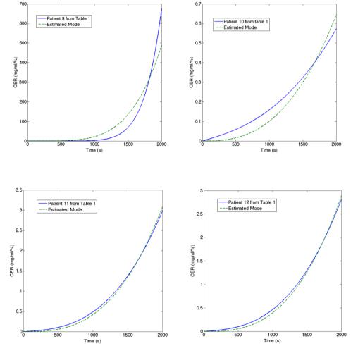
The results of the model identification from (5) are given in figures 6-11. Notice that somewhat less accurate model is identified for patient 9 and patient 10. Looking back in Table 1, these patients have the highest, respectively the lowest values for the Gamma parameter, which give the slopes of the Hill curve in Figure 5. Correlating this with the results of the identification from Figure 12, we observe that also the highest, respectively the lowest value for the n parameter is obtained for the same patients. We conclude that the n parameter holds a similar significance in (6) as that of the Gamma parameter in (5).

Figure 6. Illustration of identification result for Patient 1 and Patient 2 from Table 1.

Discussion

It may be possible to replace (5) by some form (6), since the fractional order impedance can account for time-varying dynamics by having a variable fractional order value n. This idea is a good incentive for further thought.

Complimentary Contributor Copy

Figure 7. Illustration of identification result for Patient 3 and Patient 4 from Table 1.

Figure 8. Illustration of identification result for Patient 5 and Patient 6 from Table 1.

Figure 9. Illustration of identification result for Patient 7 and Patient 8 from Table 1.

Complimentary Contributor Copy

Figure 10. Illustration of identification result for Patient 9 and Patient 10 from Table 1.

Figure 11. Illustration of identification result for Patient 11 and Patient 12 from Table 1.

It is obvious that i) closed loop control is necessary and ii) an averaged patient model will deliver sub-optimal results since they require a robust, conservative controller able to deal with the inter-patient variability. Moreover, it is also clear that the inter-patient variability may vary quite significantly and that one single controller (without online adaptation) will never suffice in practice.

A first problem is to find online adaptation algorithms which may adapt the model parameters k and n to the patient characteristics. Identification from logarithmically sampled data has been proposed in (De Keyser et al., 2011) and represents a good framework for developing the online identification algorithm.

Another problem is to find a solution to integrate the model from (6) into a closed loop control system taking into account the requirement for a logarithmic sample time (i.e., in order to maintain linearity). It has already been shown in various examples that a Riemann sampling rate (i.e., linear periodic) may be outperformed by a Lebesque sampling rate (i.e., event-triggered) in several applications (Goodwin et al., 2013). Since the Lebesque sampling rate is an event trigerred rate used successfully in practice in closed loop control (e.g.,

Complimentary Contributor Copy