


In: Fractional Calculus: Applications |
ISBN: 978-1-63463-221-8 |
Editors: Roy Abi Zeid Daou and Xavier Moreau |
© 2015 Nova Science Publishers, Inc. |
Chapter 5
FROM THE FORMAL CONCEPT ANALYSIS
TO THE NUMERICAL SIMULATION OF THE THERMAL DIFFUSION PHENOMENA IN A FINITE MEDIUM
Riad Assaf1,2, , Roy Abi Zeid Daou2,†,
Xavier Moreau1,‡ and Fady Christophy1,2,#
1University of Bordeaux, IMS Laboratory, Talence, Bordeaux, France
2Lebanese German University, Faculty of Public Health, Biomedical Technologies department, Sahel Alma, Jounieh, Lebanon
Abstract
This chapter shows the use of the fractional order approach in the study of the thermal interface behavior in view to facilitate the identification of this phenomenon and the optimization of its process control. After a short introduction, the main parameters are defined then the semi-infinite plane case study is considered. A representative model is developed based on the system equations. The operational, frequency and time responses are studied. The case study of a finite plane follows using the same methodology, nevertheless exact analytical solutions in the time domain don’t exist; their approximations will be treated in other publications.
1. Context and Problematic
In general, the development of diffusion phenomena equations naturally leads to fractional order systems (Podlubny, 2002). There are many examples in the fields of physics such as electrochemistry (Kuhn, 2005), electromagnetism (Benchellal, 2005) (Canat, 2005), or thermal (Agrawal, 2004) (Battaglia, 2001) (Kusiak, 2005).
E-mail addresses: riad.assaf@u-bordeaux.fr; r.assaf@lgu.edu.lb.
† E-mail address: r.abizeiddaou@lgu.edu.lb.
‡ E-mail address: xavier.moreau@u-bordeaux.fr.
# E-mail addresses: fady.chrystophy@u-bordeaux.fr; f.christophy@lgu.edu.lb.
Complimentary Contributor Copy
94 |
Riad Assaf, Roy Abi Zeid Daou, Xavier Moreau et al. |
|
|
Actually, the recognition of fractional order behavior when identifying physical systems flourished starting the second half of the twentieth century (Oldham, 1974). One of these fields where the fractional order integration can show up is the thermal diffusive interfaces. In fact, for some special conditions, an integration of order 0.5 appears when identifying such system (Abi Zeid Daou, 2012, Assaf, 2012). The objective of this chapter is to study the presence of the fractional order and its effects on the system behavior, and to determine the relation between the applied flux, the conduction and the point of measurement of the temperature in a plane medium.
This objective is a milestone towards the definition of valid approximations for reliable numerical simulations of the thermal diffusion phenomena in a finite medium where exact analytical time response solutions don’t exist. For instance, one can define conditions for which a finite medium can be considered as a semi-infinite medium, and can define other conditions for which analytical approximations generate accurate time response simulations.
The understanding of the thermal diffusion phenomena, hence the establishment of a validation model has two main goals:
-As part of the identification process: to facilitate the definition of the model structure, and to pass from a black box approach to a gray box approach.
-As part of a process control model: to deduct from the validation model not only a nominal model of synthesis, but also structural and parametric uncertainties.
This chapter contains six main paragraphs other than the Abstract and the Introduction at the beginning; the Conclusion and the References at the end. A reminder of the main physical characteristics needed to describe the thermal diffusion are found in Para 2, in Para 3 a model of the diffusion phenomena in the semi-infinite medium is developed, then the relative operational, frequency and time responses are studied in Para 4. In Para 5 a model of the diffusion phenomena in the finite medium is developed, then only the corresponding operational and frequency responses are studied in Para 6 since no exact analytical solutions exist to represent the time response for the finite medium. In Para 7 one can find some step responses using Simulink, it opens the door for the need for simple and accurate approximations.
2. Parameters and Definitions
The main thermal parameters and definitions characterizing any thermal interface are presented in this paragraph.
|
Heat flow in the |
direction is represented by |
( |
). |
|
|
|
Heat flux in the |
direction is represented by |
( |
⁄ ). |
|
|
|
Thermal conductivity ( |
) [Özişik, 1980] is the material property which |
||||
|
controls the rate of heat flow in the medium. For aluminum |
. |
||||
Homogeneous and Isotropic medium [Özişik, 1980] is a material in which thermal conductivity is independent of direction.
Density of a material is represented by |
( ⁄ ). For aluminum |
⁄ . |
|
Complimentary Contributor Copy

|
|
From the Formal Concept Analysis to the Numerical Simulation … |
95 |
|||||||||
|
|
|
|
|
|
|
|
|
||||
|
Specific heat capacity |
( |
|
) is [Schneider, 1957] the heat energy |
||||||||
|
required to raise the temperature of a unit weight of the material by one degree. For |
|||||||||||
|
aluminum |
|
|
|
. |
|
|
|
|
|||
|
Thermal diffusivity |
( |
⁄ ) of a medium [Özişik, 1980] is associated with the |
|||||||||
|
speed of propagation of heat into the solid during changes of temperature with time. |
|||||||||||
|
For aluminum |
|
|
|
|
|
⁄ . |
|
|
|
||
|
|
|
|
|
|
|
|
|
||||
|
Thermal effusivity |
( |
|
) is [de Wit, 2009] a measure of the material’s |
||||||||
|
ability to exchange |
thermal |
energy |
with its surroundings. For |
aluminum |
|
||||||
|
|
|
|
|
|
|
. |
|
|
|
||
|
√ |
|
|
|
|
|
|
|||||
|
Volumetric heat capacity |
|
( |
). |
is a |
variant of |
the |
|||||
|
volumetric heat capacity [US Army, 1988]; it describes the ability of a given volume |
|||||||||||
|
(crossed by a heat flux through its area |
along its length |
) of finite medium to store |
|||||||||
|
internal energy while undergoing a temperature change. |
|
|
|
||||||||
3. Semi-Infinite Plane
We consider a semi-infinite, homogeneous, isotropic, one-dimensional plane medium of
conductivity , diffusivity |
and of initial temperature zero all over the medium (Figure 1) |
[Sabatier, 2008]. A heat |
flux ( ) is normally applied on its surface. Consequently, a |
temperature gradient ( |
) appears, which is a function of the independent time variable |
as well as the abscissa |
of the temperature measurement point, inside the medium. |
Figure 1. Diffusion in a semi-infinite plane medium.
3.1. System Definition
The one-dimensional heat conduction equation (Özişik, 1985) is given by a partial differential equation:
( ) |
( ) |
. |
(1) |
|
|
|
|
||
|
|
|
||
Since the initial temperature is zero all over the medium:
( |
) |
(2) |
The Fourier law states the boundary condition (Özişik, 1985) where the flux is applied, the second condition is trivial:
Complimentary Contributor Copy

96 |
Riad Assaf, Roy Abi Zeid Daou, Xavier Moreau et al. |
|
|
( |
) |
( ) |
; |
|
|
|
(3) |
||
|
|
|||
|
|
|
|
|
( |
) |
. |
|
(4) |
3.2. System Resolution
The use of the fractional calculus to resolve the problems of the diffusive interfaces dates back to the beginning of the 20th century [Battaglia, 2001]. The system of (Eq. 1-4) represents
the relations that model this interface knowing that the input signal is the flux |
( ) whereas |
|||||||
the output signal is the temperature |
( |
) as shown in Figure 1. |
|
|||||
The initial condition of the temperature being zero, Laplace transform * + of (Eq. 1) is: |
||||||||
|
̅( ) |
|
|
̅( |
) |
where ̅( ) |
* ( )+. |
(5) |
|
|
|
|
|||||
|
|
|
||||||
This is a differential equation of the 2nd order in x. Its general solution is:
̅( |
) |
( ) , |
(6) |
leading to the characteristic equation:
( ) |
|
, |
(7) |
|
which has the following 2 roots ( ) and ( ):
√ |
|
* + |
(8) |
|
Hence the solution of (Eq. 5) is:
̅( ) |
|
|
|
|
|
( ) √ ⁄ |
( ) √ ⁄ |
(9) |
|||
Resolving (Eq. 9) for the boundary conditions (Eq. 3-4) gives the values of ( ), let:
( |
) |
|
|
|
{ ( ) |
|
|
|
̅( ) |
|
√ |
|
||
|
|
|||
|
|
|
|
|
|
|
|||
( ) and
(10)
Taking into consideration the definitions of the characteristic parameters and the outcome of (Eq. 10) then resolving (Eq. 9), the solution of (Eq. 5) is found to be:
̅( ) |
|
|
|
|
|
|
|
|
|
√ ⁄ |
̅( ). |
(11) |
|||
|
|
||||||
√ |
|||||||
|
|
|
|||||
Complimentary Contributor Copy
From the Formal Concept Analysis to the Numerical Simulation … |
97 |
|
|
Under the assumption of an initial condition of the temperature being zero, the transfer function ( ) between the input flux ̅( ) and the output temperature ̅( ) is:
( )
or rewritten as:
̅( ) |
|
|
|
|
|
|
||
|
|
√ ⁄ |
, |
(12) |
||||
|
|
|
|
|
||||
̅( ) √ |
|
|||||||
|
|
|
|
|||||
|
|
|
|
|
|
|||
|
( |
) |
|
|
|
|
( |
) ( |
|
|
), |
(13) |
||||||||||||
with the following considerations: |
|
|
|
|
|
|
|
|
|
|
|
|
|
|
|
|
|
|
|
|
|
|||
|
|
|
|
|
|
̅( |
) |
|
|
|
|
|
|
|
|
|
|
|
|
|
|
|||
|
|
|
|
|
|
|
|
|
|
|
|
|
|
|
|
|
|
|
|
|
|
|
|
|
|
|
|
|
|
|
̅( ) |
|
|
|
|
|
|
|
|
|
|
|
|
|
|
|
|
||
|
|
|
|
|
|
|
|
|
√ |
|
|
|
|
|
|
|
|
|
||||||
|
|
|
|
( |
|
) |
|
|
|
̅( |
) |
|
|
|
|
|
|
|
|
(14) |
||||
|
|
|
|
|
|
|
|
|
|
|
|
|
|
|
|
|
|
|
|
|||||
|
|
|
|
|
|
|
̅( |
) |
|
|
|
|
|
|
|
|||||||||
|
|
|
|
|
|
|
|
|
|
|
|
|
|
|
|
|
|
|
|
|||||
|
{ |
( |
) |
|
̅( |
) |
. |
|
|
/ |
|
|
|
|
|
|
||||||||
|
|
|
|
|
|
|
|
|
|
|||||||||||||||
|
|
|
|
|
|
|
|
|
|
|
|
|
|
|
|
|
|
|||||||
|
|
̅( |
) |
|
|
|
|
|
|
|
|
|
|
|
|
|
|
|||||||
and defining a cutoff frequency |
as: |
|
|
|
|
|
|
|
|
|
|
|
|
|
|
|
|
|
|
|
|
|||
|
|
|
|
|
|
|
|
|
|
⁄ |
. |
|
|
|
|
|
|
|
|
(15) |
||||
Consequently, the transfer function |
|
( |
|
|
) of the system can be seen as three cascading |
|||||||||||||||||||
functions represented in Figure 2. |
|
|
|
|
|
|
|
|
|
|
|
|
|
|
|
|
|
|
|
|
|
|||
|
|
|
|
|
H x, s |
|
|
|
|
|
|
|
|
|
|
|
|
|
||||||
|
|
|
|
|
|
|
|
|
|
|
|
|
|
|
|
|
|
|
|
|
||||
|
|
|
s0.5T 0, s |
|
|
|
|
|
|
|
|
|
|
|
|
|
|
|
T x, s |
|||||
s |
|
|
|
|
|
|
|
|
|
|
|
T 0, s |
|
|
|
|
|
|
||||||
|
|
|
|
|
|
|
|
|
|
|
|
|
|
|
|
|
||||||||
|
|
|
|
|
|
|
|
|
|
|
|
|
|
|
|
|
|
|
|
|
|
|
|
|
|
|
|
|
|
|
|
|
|
|
|
|
|
|
|
|
|
|
|
|
|
|
|
|
|
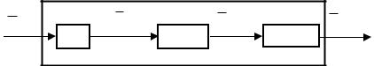
Figure 2. Block diagram illustrating the transfer function ( |
) of the semi-infinite medium. |
|
||||||
The function |
depends on the medium physical characteristics, it links the input flux |
|||||||
̅( ) and the fractional derivative of order |
of the temperature at |
. |
|
|||||
Then, |
( ) is a fractional integrator of order |
that gives the temperature at |
. |
|||||
The last function ( |
) generates the output temperature ̅( |
) at any point of the |
||||||
semi-infinite medium.
This new approach allows understanding the link existing between the two kinds of study encountered in the dynamics of thermal systems, i.e.:
- |
When the boundary condition at |
is the flux ̅( ); it is recognized as Neumann |
|
(second-type) boundary condition. |
|
- |
When the boundary condition at |
is the temperature ̅( ); it is recognized as |
Dirichlet (first-type) boundary condition.
Complimentary Contributor Copy