5.Relationship of Rabotnov Fractional Operators with Other Fractional Operators

Along with Rabotnov fractional operators there are exist other fractional operators which are used to solve different problems of viscoelasticity. In this Section, we consider those fractional operators which are somehow or other connected with Rabotnov operators.

5.1.Rzhanitsyn Operator

Let us consider Boltzmann-Volterra relationships with different kernels of relaxation Kε and retardation Kσ

As a hereditary kernel we chose Rzhanitsyn kernel [71]

which could be both the kernel of relaxation and the kernel of retardation, although Rzhanitsyn himself used it only as the creep kernel [72].

Putting i = σ in (118) and substituting it in (117), we have

In order to reverse from the frequency domain to the time domain in relationship (122), it is necessary to calculate the integral

Complimentary Contributor Copy

Reversing from the frequency domain to the time domain in (122) with due account for (125), finally we obtain

(126) If we reverse from the image to the original in (121) considering the expansion of the

function (1 + pτσ)−γ in a series

involves the fractional-exponential function, the attenuation of which with time is strengthened by decaying exponent.

If we take the Abel kernel as Kσ kernel

tγ−1

Kσ(t) = (γ)τσγ ,

Complimentary Contributor Copy

Relationship (129) is equivalent to the Maxwell model, wherein ordinary timederivatives are substituted by fractional derivatives.

Although Rzhanitsyn fractional operator (1 + τσ d/dt)−γ entering in (127) does not involve the fractional derivative in the explicit form, as Rabotnov operator [1+τσγ (d/dt)γ)−1] does, however, as it will be shown below on the example of a viscoelastic oscillator, possesses similar features.

the features of which have been studied in [59].

From (130) it is evident that the combinational Rabotnov-Rzhanitsyn operator (130) at β = 1 goes over into the Rabotnov operator, while at α = 1 it transforms into the Rzhanitsyn operator, respectively.

5.2.Koeller Viscoelastic Models

In 1986 Koeller suggested two viscoelastic models involving fractional derivatives with several fractional parameters and several relaxation (retardation) times [34]

where ai, bj and βi, γj (i, j = 1, 2, ..., n) are certain coefficients, 0 < γ < 1 is the fractional parameter, E∞ = an/bn, and

is the Riemann-Liouville fractional derivative [55].

Complimentary Contributor Copy

The model (132) is equivalent to the model (131). In order to show this, it is necessary to find the roots of equations

and suppose that all of them are simple real negative roots Zj = −t−j α = −γj (j = 1, ..., n) and Yi = −τi−α = −βi (i = 1, ..., n), and they are different in magnitude. Knowing the roots, it is possible to change the sums in (131) by the products.

However, the thermodynamic analysis of the models (131) and (132) was not carried out, what did not allow Koeller [34] to determine the physical meaning of the involving parameters, as well as to define the admissible boundaries of their domains.

Such analysis was performed in Rossikhin and Shitikova [62, 63, 65, 67], wherein it has been shown that the both models (131) and (132) could be reduced to the generalized Rabotnov model under the appropriate choice of entering constant values. Moreover, only with such a choice of the constants the both models become to be thermodynamically admissible. Really, the model (132) could be rewritten as

6=j)

The value Pn Aj = 1, since the operator Dγn with the coefficient equal to unit enters

j=1

into the numerator and denominator of the fraction in the left-hand side of formula (135). Considering formula (10), from (135) we have

Complimentary Contributor Copy

As a result we are led to generalized Rabotnov’s rheological equation with the operator (23).

Putting ε = ε0 = const in (137), we obtain the relationship

is Mittag-Leffler function.

Tending t to ∞ in (138) and considering that in so doing Eγ [− (t/tj )γ ] tends to zero,

and expand the fraction in the right-hand side of (141) in simple fractions

Complimentary Contributor Copy

the rheological parameters by reducing the given model involving fractional derivatives to the known Rabotnov model, representing itself Boltzmann-Volterra relationships with the sum of 3γ -operators which possess one fractional parameter and several relaxation (retardation) times, namely: the values τi−γ and t−j γ should alternate with each other (32) as it is shown in Fig. 1.

In other words, in order the models (137) and (143) are to be resolvent, as it has been shown by Rabotnov [48], it is necessary that the relaxation times τi−γ and the retardation times t−j γ should obey the inequalities according to (32).

˜ ˜

In conclusion it should be noted that if any two hereditarily elastic operators, K and E,

or and ˜, as examples, are given in terms of the Rabotnov-type operators, then it is rather

µ˜ E

easy to determine all other operators of the model under consideration, which depend on the two given viscoelastic operators.

6.Free Vibrations of Oscillators on the Basis of Fractional Operator Viscoelastic Models

Assume that viscoelastic features of operators are described by the Bolzmann-Volterra relationships with the relaxation kernel Kε(t) and retardation kernel Kσ(t). Then the equations of motion of such an oscillator could be written in two different but equivalent forms

Complimentary Contributor Copy

Figure 2. Contour of integration.

where x is the coordinate, F is the amplitude of force impulse per unit mass, ω∞ is the frequency of elastic vibrations corresponding to the nonrelaxed magnitude of the elastic

The solution of (149) in the time domain according to the inversion Mellin-Fourier formula has the form

Functions x¯(p) considered here are multi-valued functions with the branch points p = 0 and p = −∞ or p = −s , s ≥ 0 and p = −∞. In other words, the inversion should be carried out on the first sheet of Riemannian surface with a cut along the real negative semiaxis from 0 to −∞ or from −s to −∞. Figure 2 shows the closed contour of integration for the function with the branch points p = 0 and p = −∞. If a function possesses the branch points p = −s and p = −∞, then the center of a small circumference should locate at the point p = −s . Due to the Jordan lemma, the curvilinear integrals taken along the arcs cR tend to zero at R → ∞. For weakly singular kernels, the integral taken along cρ also tends to zero when ρ → 0. Besides, the function x¯(p) possesses the ordinary poles at the same magnitudes of p which vanish the denominator in the formula (149), i.e., they

Complimentary Contributor Copy

From relationships (157) and (158), we find the values of r and ψ which are, respectively, the modulus and argument of the root of characteristic Eqs. (151) and (152).

Using the Jordan lemma and the main theorem of the theory of residues, the solution to Eqs. (157) and (158) may be written as

where H(s−s ) is the Heaviside function, the summation is taken over all isolated singular points (poles).

Since characteristic equations possess, as a rule, two complex conjugate roots

Complimentary Contributor Copy

and B(τ ) is the function of distribution of the relaxation parameters (retardation parameters) of the dynamic system.

From Eq. (162) it is seen that the relationship describing vibrations of an oscillator with the natural frequency ω and the damping factor α possesses two terms, one of which describes the drift of the equilibrium position and is represented by the integral involving the distribution function of dynamic and rheological parameters, while the other term is the product of two time-dependent functions, exponent and sine, and it describes damped

vibrations around the drifting equilibrium position, in so doing the drift is defined by the function A0(t). The first term xdrift(t) is governed by an improper integral taken along two

sides of the cut along the negative real semi-axis of the complex plane (see Fig. 2), while the second term xvibr(t) is determined by two complex conjugate roots of the characteristic equation, which locate in the left half-plane of the complex plane.

The original method for solving characteristic equation with fractional powers without its rationalization has been suggested in [40, 89], when the roots and model’s parameters (relaxation or retardation times) are found at a time. It has been established that the characteristic equation lacks real negative roots and possesses only two complex conjugate roots. The behavior of the characteristic equation roots in the complex plane depends on the type of relaxation or creep kernel involved in the model of an oscillator under consideration. The interested reader is referred to Refs. [55, 60, 64] for a fully comprehensive description of the mathematical formulation.

Note that 25 years later than it was published in [40, 89], this result was re-discovered in [7].

Thus, in order to obtain the final solution, it is necessary to specify the type of the relaxation or creep kernel. Below we consider a few such examples.

6.1.Rabotnov Model

If we use the Rabotnov model as a relaxation kernel (16), then the solution (159) takes the form of (162) [57], where

a = (2 + γ)r1+γ cos(1 + γ)ψ + 2τ −γ r cos ψ + γω∞2 rγ−1 cos(γ − 1)ψ, b = (2 + γ)r1+γ sin(1 + γ)ψ + 2τ −γ r sin ψ + γω∞2 rγ−1 sin(γ − 1)ψ,

and ω0 is the frequency of elastic vibrations corresponding to the relaxed magnitude of the elastic modulus.

Complimentary Contributor Copy

The behavior of the roots of the characteristic equation (151) as function of the parameter τ −γ is shown in Figs. 3 a-d for ω∞ = 1 and four values ξ = 0, 1/50, 1/9 and 1/6, respectively, where figures near curves denote the magnitudes of the value γ, and

ξ = E0/E∞ = 1 − ν .

Figure 3. Behavior of the complex conjugate roots p1,2 = −α ± iω for an oscillator based on the Rabotnov model: (a) ξ = 0, (b) ξ = 1/50, (c) ξ = 1/9, and (d) ξ = 1/6.

It is seen that the τ −γ -dependence of the two complex conjugate roots p1,2 = −α ± iω at γ 6= 1leave the points ±i and converge in the points ±iξ1/2 when τ −γ changes from

Complimentary Contributor Copy

0 to ∞; in so doing it does not meet the real negative semi-axes and remains inside the curves for the τ −γ -dependencies of three roots of the characteristic equation with γ = 1 (the ordinary standard linear solid model). The behavior of the two roots of three at γ = 1 (the third root is the real root all the time and changes from 0 to ∞ as τ −γ varies from 0 to ∞) essentially depends on the magnitude of the value ξ. Thus, at the values ξ taken from the interval (0, 1/9) the two complex conjugate roots first become real as τ −γ changes from 0 to ∞. But then during further increase in τ −γ , they again become complex conjugate roots, i.e., the domain of aperiodicity (the values of τ −γ wherein ω = 0) has finite dimensions contracting with increase in ξ (Figs. 3a,b). At ξ = 0 the ordinary Maxwell model with a semi-infinite domain of aperiodicity is obtained (Fig. 3a) [57], but at ξ = 1/9 the domain of aperiodicity degenerates into a point (Fig. 3c). When ξ > 1/9, the domain of aperiodicity completely disappears (Fig. 3d).

In other words, at γ 6= 1the behavior character of the roots of the characteristic equation for the Rabotnov model is governed by the magnitudes of the value ξ, which may be considered as the deficiency of the elastic modulus.

6.2.Rzhanitsyn Model

It has been already mentioned in Sect. 5.1 that the Rzhanitsyn kernel (118) [71] could be utilized as the kernel of relaxation and the kernel of retardation, so we will consider these two cases separately.

6.2.1.Rzhanitsyn After-effect Kernel

Hereditary elastic oscillator model with the Rzhanitsyn creep, or after-effect, kernel (120) was studied in [56], wherein it had been shown that knowing the behavior of roots of the characteristic equation (152) and considering that the branch points are s = τσ−1 and −∞, the solution (159) may be written in the form of (162) with

h = 2rRγ cos(ψ+Φ)+r2Rγ−1 γτσ cos[2ψ+(γ−1)Φ]+τσω∞2 γRγ−1 cos(γ−1)Φ+2rνσ cos ψ, q = 2rRγ sin(ψ+Φ)+r2Rγ−1γτσ sin[2ψ+(γ−1)Φ]+τσω∞2 γRγ−1 sin(γ−1)Φ+2rνσ sin ψ, and

Dσ(τ ) = τ γ (1 + ω∞2 τ 2)−1(τσ − τ )−γ νσ .

The root locus in the complex plane as function of the parameter τσ for three magnitudes νσ = 49, 8, and 5 (ξ = 1/50, 1/9 and 1/6) at ω∞ = 1 was presented in Figs. 2a-c in [56]. Its analysis reveals that the behavior of the characteristic equation roots in the case under consideration is identical to that of the oscillator with the Rabotnov relaxation kernel shown in Figs. 3b-d for the corresponding magnitudes of the parameter ξ.

Complimentary Contributor Copy

6.2.2.Rzhanitsyn Relaxation Kernel

Let us take the Rzhanitsyn kernel (118) at i = as the relaxation kernel in the Boltzmann-Volterra relationships (116). Then the characteristic equation (151) takes the form

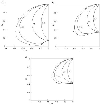
The behavior of the roots of the characteristic equation (168) in the complex plane as function of the parameter τ for four magnitudes ν = 0.98, 14/15, 8/9, and 5/6 (ξ = 1/50, 1/15, 1/9 and 1/6) at ω∞ = 1 is presented in Figs. 4(a),(b),(c), and (d), respectively, wherein the magnitudes of γ are indicated by figures. Reference to Figs. 4 shows that as τ changes from 0 to ∞, the curves for two complex conjugate roots p1,2 = −α ± iω at any 0 < γ < 1 issue out of the points ±iξ1/2 and converge at the points ±i. At ν = 0.98 and 0.12 ≤ γ < 1 (Fig. 4(a)) or ν = 14/15 and 0.47 ≤ γ < 1 (Fig. 4(b)) the domain of aperiodicity is observed, which narrows with decrease in γ from 1 to 0.12 or from 1 to 0.47 and degenerates into a point at γ = 0.12 or γ = 0.47. This domain disappears completely at 0 ≤ γ < 0.12 or 0 < γ < 0.47, respectively. At ν = 8/9 (Fig. 4(c)) and 5/6 (Fig. 4(d)) the domain of aperiodicity is entirely absent, although the domain of aperiodicity at ν = 8/9 and γ = 1 exists in the form of a point.

In other words, the structural parameter γ along with the parameter ξ influences not only the dimensions of the aperiodicity domain, but the existence of this domain as well. This circumstance profitably distinguishes the model under consideration from the previous model, since it allows one to use this model for describing dissipative processes of high intensity.

Now knowing the behavior of roots of the characteristic equation (168) and considering that the branch points are s = τσ−1 and −∞, the solution (162) is as follows [56]:

for the domains of vibration motions (one real and two complex conjugate roots)

i=1

for the boundaries of the domain of aperiodic motions (one real root, for example, β1 is the simple root, and the other real root β = β2 = β3 is one repeated root)

or (in the case, if the domain of the aperiodic motions degenerates into a point, the real root β = β1 = β2 = β3 becomes a 3-fold root)

Complimentary Contributor Copy

Figure 4. Behavior of the complex conjugate roots p1,2 = −α ± iω for an oscillator based on the fractional calculus model with the Rzhanitsyn relaxation kernel: (a) ξ = 1/50, (b) ξ = 1/15, (c) ξ = 1/9, and (d) ξ = 1/6.

Complimentary Contributor Copy

where α1, βi (i = 1, 2, 3), β and β are the real roots of Eq. (168) which are located between τ −1(1 − ν1/γ ) and the branch point τ −1, and α2 ± iω are the complex conjugate roots of Eq. (168).

terms of the damping coefficients α1, α2, βi, β, β and natural frequency ω as follows:

l1 = β2τ 3(2 + γ)(1 + γ)γ − 6βτ 2(1 + γ)γ + 4τ (1 + γ) + γ(γ − 1)(γ − 2)τ 2ω∞2 .

The value A0(t) is determined by Eq. (162), wherein the distribution function B(τ, τ ) of the relaxation and creep parameters of the dynamical system under consideration has the form

D (τ ) = τ γ (1 + ω∞2 τ 2)−1(τ − τ )−γ ω∞2 ν .

Comparison studies of damped vibrations of the hereditary elastic oscillators, whose hereditary properties are described by the fractional calculus models with the weakly singular Rzhanitsyn kernel, allow us to make the following conclusions: (1) the peculiarity of the vibrational process of the viscoelastic single-mass systems, which are modeled by the fractional calculus models with the weakly singular Rzhanitsyn kernel as the creep kernel, resides in impossibility of the transition from the vibrating motions to the aperiodic regime in spite of the known fact that under the sufficiently large intensity of dissipative processes real vibrating systems may experience the aperiodic regime; (2) the more complicated rheological model, i.e., the model with the weakly singular Rzhanitsyn kernel as the relaxation kernel, utilized for describing the viscoelastic properties of a single-mass system, allows one to trace the influence of the fractional operator parameter γ on the dynamic characteristics of the system not only in the region of vibration, but in the domain of the aperiodic motions as well. Moreover, it has been shown that the occurrence or vanishing of the region of the aperiodic motions for the model put forward is governed not only by the magnitudes of the value ν , but by the magnitudes of the value γ as well.

Complimentary Contributor Copy

6.3.Combinational Rabotnov-Rzhanitsyn Model

The comparison between theoretical and experimental results in the field of application of fractional calculus models in viscoelasticity carried out in [59] has shown that the fractional models with more than one fractional parameters seem to be very flexible for describing relaxation (retardation) behavior over wide frequency ranges and for different materials. One distinct advantage of the fractional calculus models is their ability to describe real material behavior using only a small number of parameters.

However, the analysis of many of such models [59] revealed the fact that at some magnitudes of rheological parameters they are not thermodynamically admissible, i.e., the loss tangent takes on negative values in some frequency domain and the relaxation (retardation) function becomes non-monotonic in some time intervals.

It has been proved in [59] that the rheological models involving fractional operators (130) with two independent fractional parameters 0 < α, β ≤ 1, which represent the com-

are thermodynamically well-conditioned at all magnitudes of the rheological parameters. Note that the models (175) and (176) at 0 < α, β < 1 are not resolvent despite of the

Rabotnov models at 0 < α < 1 and β = 1.

Havriliak and Negami [26, 27] used these models for the analysis of dielectric and mechanical dispersion for five polymers (polycarbonate and polyisophthalat on the basis of bisphenol A, isotaclic polymethyl methacrylate, polymethylacrylate, and co-polymers of phenylmethacrylate and acrylonitrile), while Hartmann et al. [25] utilized them for approximation of the loss factor for polymer relaxation on the basis of experimental data for different polymers. It has been shown close agreement between theoretical and experimental findings.

6.3.1.Rabotnov-Rzhanitsyn Relaxation Kernel

Now let us first consider viscoelastic oscillators (147), the behavior of which is described by the model (175), following Rossikhin and Shitikova [59]. For this case, Eq. (149) takes the form

To determine the poles of the function x¯(p) (177), it is necessary to find the roots of the characteristic equation

1 for three magnitudes of νε = 0.98, 8/9, 5/6 and β = 0.98 is presented in Figures 5 (a)-(c), respectively, where figures near curves denote the magnitudes of the fractional

Complimentary Contributor Copy

Figure 5. Behavior of the complex conjugate roots p1,2 = −α±iω for an oscillator based on the fractional calculus model with the Rabotnov-Rzhanitsyn relaxation kernel at ω∞ = 1:

(a) νε = 0.98, (b) ξ = 8/9, and (c) ξ = 5/6 when β = 0.98.

parameter α. From Figure 5 it is seen that the curves describing the roots behavior do not cut the real axis, i.e., the fundamental possibility for the transition of the vibrational process to an aperiodic regime is absent. Note that at α = 1 and fractional β this model, as it has been discussed above in Sec. 6.2.2, behaves similarly to the standard linear solid model with derivatives of an integer order, that is, the system may be both in vibrational and aperiodic regimes depending on the magnitudes of the parameter τε.

Knowing the behavior of the characteristic equation roots, the solution (159) takes the form of (162) [55], where

h = 2rRβε cos(ψ + βΦε) + r1+ααβτεαRβε −1 cos[(β − 1)Φε + (α + 1)ψ] +ω∞2 rα−1αβτεαRβε −1 cos[(β − 1)Φε + (α − 1)ψ],

Complimentary Contributor Copy

202 Yury A. Rossikhin and Marina V. Shitikova

q = 2rRβε sin(ψ + βΦε) + r1+ααβτεαRβε −1 sin[(β − 1)Φε + (α + 1)ψ] +ω∞2 rα−1αβτεαRβε −1 sin[(β − 1)Φε + (α − 1)ψ],

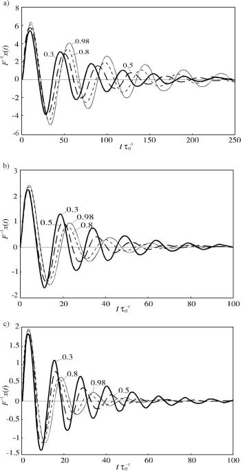
The character of the solution x(t) is presented in Figure 6, where figures near curves denote the magnitude of the fractional parameter α.

6.3.2.Rabotnov-Rzhanitsyn Retardation Kernel

Now let us consider viscoelastic oscillators (148), the behavior of which is described by the model (176), following Rossikhin and Shitikova [59]. For this case, Eq. (149) takes the

To determine the poles of the function x¯(p) (180), it is necessary to find the roots of the

The behavior of the roots in the complex plane as function of the parameter τσ is presented in Figs. 7 for three magnitudes of νσ = 49, 8 and 5, respectively, when β = 0.98.

Knowing the behavior of the characteristic equation roots, the solution (159) takes the

h = 2rRβσ cos(ψ + βΦσ) + r1+ααβτσαRβσ−1 cos[(β − 1)Φσ + (α + 1)ψ] +ω∞2 αβτσαrα−1Rβσ−1 cos[(β − 1)Φσ + (α − 1)ψ] + 2rνσ cos ψ,

q = 2rRβσ sin(ψ + βΦσ) + r1+ααβτσαRβσ−1 sin[(β − 1)Φσ + (α + 1)ψ] +ω∞2 αβτσαrα−1Rβσ−1 sin[(β − 1)Φσ + (α − 1)ψ] + 2rνσ sin ψ,

The character of the solution x(t) is presented in Figure 8, where figures near curves denote the magnitude of the fractional parameter α.

Complimentary Contributor Copy

Figure 6. Character of the solution x(t) behavior for an oscillator based on the fractional calculus model with the Rabotnov-Rzhanitsyn relaxation kernel at ω∞ = 1: (a) νε = 0.98,

(b) νε = 8/9, and (c) νε = 5/6 for β = 0.98 and τε = 1.

As it has been noted in Sec 6.2.1, when α = 1 and β = γ, the model under consideration goes over into the oscillator model with the Rzhanitsyn retardation operator, for which the behavior of the characteristic equation roots resembles the character of the roots behavior for the generalized standard linear solid model with the only difference that in this case the

Complimentary Contributor Copy

noticeable asymmetry is observed in the behavior of the roots.

Figure 7. Behavior of the complex conjugate roots p1,2 = −α±iω for an oscillator based on the fractional calculus model with the Rabotnov-Rzhanitsyn retardation kernel at ω∞ = 1:

(a) νσ = 49, (b) νσ = 8, and (c) νσ = 5 when β = 0.98.

6.4.Generalized Rabotnov Model

The equation of motion of an oscillator, hereditary features of which are described by the model (137) has the form [63]:

Applying the Laplace transformation to Eq. (183) yields

Complimentary Contributor Copy

Figure 8. Character of the solution x(t) behavior for an oscillator based on the fractional calculus model with the Rabotnov-Rzhanitsyn retardation kernel at ω∞ = 1: (a) νσ = 49,

(b) νσ = 8, and (c) νσ = 5 for β = 0.98 and τσ = 1.

Complimentary Contributor Copy

The solution in the time domain is determined by the Mellin-Fourier inversion formula (150). To calculate the integral in (150), it is necessary to determine all singular points of the complex function (184). This function has the branch points p = 0 and p = ∞ and simple poles at the same magnitudes of p which vanish the denominator of formula (184), i.e., they are the roots of the characteristic equation

Since for the multivalued functions possessing branch points the inversion formula is valid only for the first sheet of the Riemann surface, then for calculating integral (150) we shall use the closed contour presented in Fig. 2. Using the main theorem of the residue

theory, it could be written in the form of (159).

The value xdrift(t) in (159) is calculated immediately and has the form [63]

In order to calculate xvibr(t), it is necessary to investigate the roots of the characteristic equation (185). It has been proved in [63] that (185) lacks real roots and possesses for each fixed magnitude of tj (j = 1, ..., n) only two complex conjugate roots p1,2 = −δ ± iω. For example, in the case of n = 2, the character of the root locus behavior as function of Z1(t1) = (rt1)γ at fixed magnitudes of Z2(t1) = (rt2)γ is shown in Figs. 9 for ξ = 1 − (m1 + m2) = 1/9 at m1 = m2 = 4/9. The values of the fractional parameter γ are indicated by digits near the corresponding curves. In all Figs. 9 a-f only one from each pair of complex conjugate roots is shown in the upper quadrant of the negative half-plane of the complex plane.

Knowing the behavior of the characteristic equation roots, the function xvibr(t) could be represented as