

106 |
Riad Assaf, Roy Abi Zeid Daou, Xavier Moreau et al. |
|
|
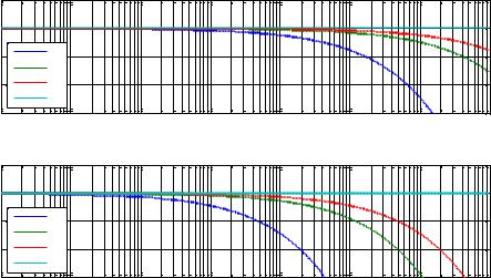
Note that, as long as the frequency of variation of the temperature is low relatively to |
|
the diffusivity , the temperature variation is uniform and harmonic. |
|
When the frequency of variation of the temperature |
increases, the diffusion depth of |
the temperature decreases in the semi-infinite medium. |
|
5. Finite Plane
We consider a finite, homogeneous, isotropic, one-dimensional plane medium of
thickness , conductivity |
, diffusivity , and of initial temperature zero all over the medium |
||
(Figure 9). A heat flux |
( ) is normally applied on its surface at |
; it is assumed that |
|
there are no losses at this point. Consequently, a temperature gradient ( |
) appears, which |
||
is a function of the independent time variable as well as the abscissa |
of the temperature |
||
measurement point, with |
, |
- inside the medium. |
|
5.1. System Definition
The one-dimensional heat conduction equation (Özişik, 1985) is given by a partial differential equation:
( ) |
( ) |
. |
(47) |
|
|
|
|
||
|
|
|
||
Since the initial temperature is zero all over the medium:
( |
) |
. |
(48) |
The Fourier law states the boundary conditions (Özişik, 1985) where the flux is applied, as well as at the second end:
( |
) |
|
( ) |
|
|
|
|
|
|
|
|
(49) |
|
|
|
|
|
|
||
|
|
|
|
|
|
|
( |
|
) |
|
. |
|
|
|
|
|
|
|
(50) |
|
|
|
|
|
|
||
|
|
|
|
|
|
|
5.2. System Resolution
The system of (Eq. 47-50) represents the relations that model the diffusive interface knowing that the input signal is the flux ( ) whereas the output signal is the temperature
( ) as shown in Figure 9. |
|
|
|
|
|
||
The initial condition of the temperature being zero, Laplace transform |
* + of (Eq. 47) is: |
||||||
|
̅( ) |
|
̅( ) |
where ̅( ) |
* ( )+ |
(51) |
|
|
|
|
|
||||
|
|
|
|
||||
Complimentary Contributor Copy
From the Formal Concept Analysis to the Numerical Simulation … |
107 |
|
|
The solution of (Eq. 51) is similar to the previous case, hence:
|
|
|
|
|
|
|
|
|
|
|
|
|
|
̅( ) |
( ) √ ⁄ |
|
( ) √ ⁄ . |
(52) |
|||||||||
Resolving (Eq. 52) for the boundary conditions (Eq. 49-50) gives the values of |
( ) and |
||||||||||||
( ), let: |
|
|
|
|
|
|
|
|
|
|
|
|
|
( ) |
( ) |
|
|
|
|
̅( ) |
|
||||||
|
√ |
|
|
||||||||||
|
|
|
|||||||||||
{ |
|
|
|
|
|
|
|
|
|
(53) |
|||
|
|
|
|
|
|
||||||||
|
|
|
|
|
|
|
|
|
|
|
|
||
( ) |
√ |
|
|
( ) |
√ |
|
|
|
|||||
|
|
|
|||||||||||
Taking into consideration the definitions of the characteristic parameters and the outcome of (Eq. 53), thus:
( ) √
{ ( ) √
then the solution of (Eq. 51) is found to be:
|
√ ⁄ |
√ ⁄ |
√ ⁄ |
|
√ ⁄ |
√ ⁄ |
√ ⁄ |
̅( )
(54)
̅( )
|
|
|
|
|
|
|
|
|
|
|
|
|
|
̅ |
|
( |
)√ ⁄ |
( )√ ⁄ |
|
|
|||||||
|
|
|
|
|
|
|
|
|
|
|
|
|
|
|
|
|
|
|
|
|
|
|
|
|
|
|
|
( ) √ |
|
|
|
√ ⁄ |
√ ⁄ |
̅( ) . |
(55) |
||||||
Under the assumption of an initial condition of the temperature being zero, the transfer
function ( ) between the input flux ̅( ) and the output temperature ̅( |
) is: |
||||||||||||||||||||||||||||||||||||
|
|
|
|
|
|
|
|
|
|
|
|
|
|
|
|
|
|
|
|
|
|
|
|
|
|
|
|
|
|
|
|
|
|
|
|
||
|
|
|
|
̅( |
) |
|
|
|
|
|
( |
|
)√ ⁄ |
( )√ ⁄ |
|
|
|||||||||||||||||||||
( |
|
) |
|
|
|
|
|
|
|
|
|
|
|
|
|
|
|
|
|
|
|
|
|
|
|
, |
|
|
|
(56) |
|||||||
|
|
|
|
|
|
|
|
|
|
|
|
|
|
|
|
|
|
|
|
|
|
|
|
|
|
|
|
|
|
|
|||||||
|
|
|
̅ |
( ) |
|
|
|
|
|
|
|
|
|
|
|
|
|
|
|
|
|
|
|
|
|
|
|
||||||||||
|
|
|
|
|
√ |
|
|
|
|
√ ⁄ |
√ ⁄ |
|
|
||||||||||||||||||||||||
|
|
|
|
|
|
|
|
|
|
|
|
|
|
|
|
|
|
|
|
|
|
||||||||||||||||
then, introducing the hyperbolic functions |
|
|
and |
|
|
|
|
|
|
|
the |
|
|
transfer |
function ( ) |
||||||||||||||||||||||
becomes: |
|
|
|
|
|
|
|
|
|
|
|
|
|
|
|
|
|
|
|
|
|
|
|
|
|
|
|
|
|
|
|
|
|
|
|
|
|
|
|
|
|
|
|
|
|
|
|
|
|
|
|
|
|
|
|
|
|
|
|
|
|
|
|
|
|
|
|
|
|
|
|
|
|
||
( |
) |
̅( |
) |
|
|
|
|
|
|
|
|
|
|
|
|
|
|
|
|
|
|
|
(( |
|
|
)√ ⁄ ) |
|
|
|||||||||
|
|
|
|
|
|
|
|
|
|
|
|
|
|
|
|
|
|
|
|
|
|
|
|
|
|
|
|
|
|
, |
(57) |
||||||
|
|
|
|
|
|
|
|
|
|
|
|
|
|
|
|
|
|
|
|
|
|
|
|
|
|
|
|
|
|
|
|
|
|
||||
̅ |
( ) |
|
|
|
|
|
|
|
|
|
|
|
|
|
|
|
|
|
|
|
|
|
|
|
|
|
|
|
|
|
|
|
|||||
|
|
√ |
|
|
|
|
|
. √ ⁄ / |
. |
√ ⁄ / |
|||||||||||||||||||||||||||
|
|
|
|
|
|
|
|
|
|
|
|||||||||||||||||||||||||||
or rewritten as: |
|
|
|
|
|
|
|
|
|
|
|
|
|
|
|
|
|
|
|
|
|
|
|
|
|
|
|
|
|
|
|
|
|
|
|
|
|
|
( |
|
) |
|
|
|
|
|
|
( ) |
( |
|
|
) ( |
|
|
) , |
|
|
|
|
|
|
(58) |
|||||||||||||
where: |
|
|
|
|
|
|
|
|
|
|
|
|
|
|
|
|
|
|
|
|
|
|
|
|
|
|
|
|
|
|
|
|
|
|
|
|
|
Complimentary Contributor Copy
108 |
Riad Assaf, Roy Abi Zeid Daou, Xavier Moreau et al. |
|
|
|
|
|
|
|
|
|
|
̅( |
) |
|
|
|
|
|
|
|
|
|
|
|
|
|
|
|
|
|
|
|
|
|
|
|
|
|
|
|
|
|||||
|
|
|
|
|
|
|
|
|
|
|
|
|
|
|
|
|
|
|
|
|
|
|
|
|
|
|
|
|
|
|
|
|
|
|
|
|
|
|
|
|
|
|
|
|
|
|
|
|
|
|
̅( ) |
|
|
|
|
|
|
|
|
|
|
|
|
|
|
|
|
|
|
|
|
|
|
|
|
|
|
|
|
|
|
||||
|
|
|
|
|
|
|
|
|
|
|
|
|
|
|
|
|
|
√ |
|
|
|
|
|
|
|
|
|
|
|
|
|
|
|
|
|
|||||||
|
|
|
|
|
( ) |
|
|
|
|
|
̅( |
) |
|
|
|
|
|
|
|
|
|
|
|
|
|
|
|
|
|
|
||||||||||||
|
|
|
|
|
|
|
|
|
|
|
|
|
|
|
|
|
|
|
|
|
|
|
|
|
|
|
|
|
|
|
|
|
|
|
|
|
|
|
|
|||
|
|
|
|
|
|
|
|
|
|
|
̅( |
|
|
|
|
) |
|
|
|
|
|
|
|
|
|
|
|
|
|
|||||||||||||
|
|
|
|
|
|
|
|
|
|
|
|
|
|
|
|
|
|
|
|
|
|
|
|
|
|
|
|
|
|
|
||||||||||||
|
|
|
( |
|
) |
|
|
̅( |
) |
|
|
|
|
|
|
|
|
|
|
|
|
|
|
|
|
|
|
|
|
|
|
|
||||||||||
|
|
|
|
|
|
|
|
|
|
|
|
|
|
|
|
|
|
|
|
|
|
|
|
|
|
|
|
|
|
|
|
|
|
|
|
|
|
(59) |
||||
|
|
|
|
|
̅( |
) |
|
|
|
|
|
|
|
|
|
|
|
|
|
|
|
|
|
|
|
|
|
|||||||||||||||
|
|
|
|
|
|
|
|
|
|
|
|
|
|
(√ ⁄ |
) |
|
|
|||||||||||||||||||||||||
|
|
|
|
|
|
|
|
|
|
|
|
|
|
|
|
|
|
|
|
|
||||||||||||||||||||||
|
|
|
|
|
|
|
|
|
|
|
|
|
|
|
|
|
|
|
|
|
|
|
|
|
|
|
|
|
|
|
|
|
||||||||||
|
|
|
|
|
|
|
|
|
|
|
|
|
|
|
|
|
|
|
|
|
|
|
|
|
|
|
|
|
|
|
|
|
|
|
|
|
|
|||||
|
|
|
( |
|
) |
|
̅( |
) |
|
|
|
|
|
|
|
|
|
|
(√ ⁄ |
) |
|
|
||||||||||||||||||||
|
|
|
|
|
|
|
|
|
|
|
|
|
|
|
|
|
|
|
|
|
|
|
|
|
|
|
|
|
||||||||||||||
|
|
|
|
|
|
|
|
|
|
|
|
|
|
|
|
|
|
|
|
|
|
|
|
|
|
|
|
|
|
|
|
|
|
|
|
|
|
|
||||
|
|
|
|
|
̅( |
) |
|
|
|
|
|
|
|
|
|
|
|
|
|
|
|
|
|
|
|
|
|
|
|
|
||||||||||||
|
|
|
|
|
|
|
|
|
|
|
|
|
|
|
|
(√ ⁄ |
) |
|
|
|
||||||||||||||||||||||
|
|
|
{ |
|
|
|
|
|
|
|
|
|
|
|
|
|
|
|
|
|
|
|
||||||||||||||||||||
|
|
|
|
|
|
|
|
|
|
|
|
|
|
|
|
|
|
|
|
|
|
|
|
|
|
|
|
|
|
|
|
|||||||||||
|
|
|
|
|
|
|
|
|
|
|
|
|
|
|
|
|
|
|
|
|
|
|
|
|
|
|
|
|
|
|
|
|
|
|
|
|
|
|
|
|
|
|
with the following considerations: |
|
|
|
|
|
|
|
|
|
|
|
|
|
|
|
|
|
|
|
|
|
|
|
|
|
|
|
|
|
|
|
|
|
|
|
|
|
|
|
|||
|
|
|
{ |
|
|
|
|
|
|
|
|
|
. |
|
|
|
|
|
/ |
|
|
|
|
|
|
|
|
|
|
|
|
|
|
|
|
|
|
(60) |
||||
|
|
|
|
|
|
|
|
|
|
|
|
|
|
|
|
|
|
|
|
|
|
|
|
|
|
|
|
|
|
|
|
|
|
|||||||||
|
|
|
|
|
|
|
|
|
|
|
|
|
|
|
|
|
|
|
|
|
|
|
|
|
|
|
|
|
|
|
|
|
|
|
|
|
|
|
|
|
||
|
|
|
|
|
|
|
|
|
|
|
|
|
|
|
|
|
|
|
|
|
|
|
|
|
|
|
|
|
|
|
|
|
|
|
|
|
|
|
|
|
||
|
|
|
|
|
|
|
|
|
|
|
|
|
|
|
|
|
|
|
|
|
|
|
|
|
|
|
|
|
|
|
|
|
|
|
|
|
|
|
||||
|
|
|
|
|
|
|
|
|
|
|
|
( |
|
|
|
|
) |
|
|
|
|
|
|
|
|
|
|
|
|
|
|
|
|
|
||||||||
One can derive from (Eq. 60) that |
|
|
|
and |
|
|
|
|
|
|
|
are linked by the following relation: |
|
|||||||||||||||||||||||||||||
|
|
|
|
|
|
|
|
. |
|
|
|
|
|
/ |
|
|
|
|
|
. |
|
|
|
|
|
|
|
|
|
|
|
|
(61) |
|||||||||
|
|
|
|
|
|
|
|
|
|
|
|
|
|
|
|
|
|
|
|
|
|
|
|
|
|
|
||||||||||||||||
One can derive also the thermal diffusion time constant defined as: |
|
|
||||||||||||||||||||||||||||||||||||||||
|
|
|
|
|
|
|
|
|
|
|
|
|
|
|
|
|
|
|
|
|
|
|
. |
|
|
|
|
|
|
|
|
|
|
|
|
|
|
|
|
(62) |
||
|
|
|
|
|
|
|
|
|
|
|
|
|
|
|
|
|
|
|
|
|
|
|
|
|
|
|
|
|
|
|
|
|
|
|
|
|
|
|
||||
To clarify, the different temperatures found in the system (Eq. 59) are as follows: |
|
|||||||||||||||||||||||||||||||||||||||||
- |
̅( |
|
) is the measured temperature at |
|
|
|
|
|
|
|
|
|
if the medium is considered to be |
|||||||||||||||||||||||||||||
|
a semi-infinite medium. |
|
|
|
|
|
|
|
|
|
|
|
|
|
|
|
|
|
|
|
|
|
|
|
|
|
|
|
|
|
|
|
|
|
|
|
|
|
|
|
||
- |
̅( |
) is the measured temperature at |
|
|
|
|
|
|
|
|
|
of the finite medium of length . |
||||||||||||||||||||||||||||||
- |
̅( |
) is the measured temperature at |
, |
|
, |
-. |
|
|
||||||||||||||||||||||||||||||||||
Consequently, the transfer function ( |
|
|
) of the system can be seen as four cascading |
|||||||||||||||||||||||||||||||||||||||
functions represented in (Figure 10). |
|
|
|
|
|
|
|
|
|
|
|
|
|
|
|
|
|
|
|
|
|
|
|
|
|
|
|
|
|
|
|
|
|
|
|
|
|
|
||||
The function |
depends on the medium physical characteristics, it links the input flux |
|||||||||||||||||||||||||||||||||||||||||
̅( ) and the fractional derivative of order |
of the temperature at |
. |
|
|||||||||||||||||||||||||||||||||||||||
Then, |
( ) is a fractional integrator of order |
|
|
|
|
|
|
|
that gives the temperature at |
. Its |
||||||||||||||||||||||||||||||||
output is the temperature ̅( |
). |
|
|
|
|
|
|
|
|
|
|
|
|
|
|
|
|
|
|
|
|
|
|
|
|
|
|
|
|
|
|
|
|
|
|
|
|
|
|
|||
The third block is the transfer function ( |
|
|
|
|
|
|
|
|
|
) between the temperatures ̅( |
) and |
|||||||||||||||||||||||||||||||
̅( |
). |
|
|
|
|
|
|
|
|
|
|
|
|
|
|
|
|
|
|
|
|
|
|
|
|
|
|
|
|
|
|
|
|
|
|
|
|
|
|
|
|
|
Complimentary Contributor Copy
|
|
|
From the Formal Concept Analysis to the Numerical Simulation … |
109 |
|||||||||||||||||||||||||||||
|
|
|
|
|
|
|
|
|
|
|
|
|
|
|
|
|
|
|
|
|
|
|
|
|
|||||||||
The fourth part is the transfer function |
( |
|
|
|
) having as input ̅( |
) and as output |
|||||||||||||||||||||||||||
the temperature ̅( |
). |
|
|
|
|
|
|
|
|
|
|
|
|
|
|
|
|
|
|
|
|
|
|
|
|
|
|
|
|
||||
|
|
|
|
|
|
|
|
|
|
|
|
|
|
H(x, s, L) |
|
|
|
|
|
|
|
|
|
|
|
|
|
|
|
|
|||
|
|
|
|
|
|
|
|
|
|
|
|
|
|
|
|
|
|
|
|
|
|
|
|
||||||||||
|
|
|
|
|
|
|
|
|
|
|
|
|
(0, s, oo) |
|
|
|
|
|
|
|
|
|
|
|
|
|
|
|
|||||
|
|
|
|
|
|
|
|
|
|
|
|
|
|
|
|
|
|
|
|
|
|
|
|
|
|
|
|
||||||
|
|
|
|
|
|
|
|
|
|
|
|
|
|
|
(0, s, L) |
|
|
|
|
|
|
|
|||||||||||
|
|
|
s0.5T |
(0, s, oo) |
|
|
|
|
|
T |
|
|
|
|
|
|
|
|
|
(x, s, L) |
|
||||||||||||
|
|
|
|
|
|
|
|
|
|
T |
|
|
|
T |
|||||||||||||||||||
|
|
|
|
|
|
|
I 0.5(s) |
|
|
|
|
|
|
|
F(0, s L) |
|
|
|
|
|
G(x, s, L) |
|
|
|
|
|
|
|
|||||
|
H0 |
|
|
|
|
|
|
|
|
|
|
|
|
|
|
|
|
|
|
|
|
||||||||||||
|
|
|
|
|
|
|
|
|
|
|
|
|
|
|
|
|
|
|
|
|
|
|
|
|
|||||||||
Figure 10. Block diagram illustrating the transfer function |
( |
) of the finite medium. |
|||||||||||||||||||||||||||||||
6. Responses in Finite Plane |
|
|
|
|
|
|
|
|
|
|
|
|
|
|
|
|
|
|
|
|
|||||||||||||
6.1. Asymptotic Behavior Analysis at |
|
|
|
|
|
|
|
|
|
|
|
|
|
|
|
|
|
|
|
||||||||||||||
At |
, |
|
( |
) |
|
|
( |
) |
|
, |
thus |
the temperature ̅( |
) of |
the finite |
|||||||||||||||||||
medium of length |
|
is given by: |
|
|
|
|
|
|
|
|
|
|
|
|
|
|
|
|
|
|
|
|
|
|
|
|
|
||||||
|
|
|
|
|
̅( |
|
) |
|
|
|
|
|
( ) |
( |
) ̅( ). |
|
|
|
|
|
|
|
(63) |
||||||||||
The transfer function ( |
|
) allows the analysis of the influence of the medium finite |
|||||||||||||||||||||||||||||||
|
|
|
|
|
|
|
|
|
|
|
|
|
|
|
|
|
|
|
|
|
|
|
|
|
|
|
|
|
|||||
character |
on the |
temperature |
at |
|
|
|
|
|
. As |
such, let the change of variable |
|
|
|
√ ⁄ . |
|||||||||||||||||||
Considering the definitions in (Para 2.) and (Eq. 60, 61), as a start the following is verified: if then , as ( ) , thus ( ) , accordingly it is found that:
|
|
|
|
|
( |
) |
|
|
( ) |
|
(64) |
||
which is a result similar to what was found in a semi-infinite medium at |
. |
||||||||||||
Now consider when |
then |
, as |
( |
) |
|
, thus: |
|
||||||
( |
) |
|
|
, accordingly it is found that: |
|
|
|
|
|
||||
|
|
|
|
|
|
|
|||||||
√ ⁄ |
|
|
|
|
|
||||||||
|
|
|
|
|
|
|
|
|
|
|
|
||
|
|
|
|
|
( |
) |
|
|
( ) |
|
(65) |
||
|
|
|
|
|
|
|
|
|
|
|
|||
|
|
|
|
|
|
|
|
|
|
|
|||
|
|
|
|
|
|
|
|
|
|
||||
√ ⁄
Once again, considering the definitions in (Para 2.) and (Eq. 60, 61), the (Eq. 65) is rewritten as:
( |
) |
|
. |
(66) |
|
Complimentary Contributor Copy
110 |
Riad Assaf, Roy Abi Zeid Daou, Xavier Moreau et al. |
|
|
Thus for high instances, corresponding to low frequencies (i.e. ), the asymptotic behavior of a finite medium is of capacitive type characterized by an integrator of order . It is different than the behavior in a semi-infinite medium characterized by a fractional
integrator of order |
. |
|
|
|
|
|
For low |
instances, corresponding to |
high |
frequencies, when |
then |
, as |
|
( |
) |
, thus: |
|
|
|
|
|
|
( |
) |
( ) |
|
(67) |
Accordingly an asymptotic fractional order behavior appears when |
between the |
|||||
input flux and the temperature at the boundary where the flux is applied; in fact, it is the same result that appears in the semi-infinite medium.
6.2. Asymptotic Behavior Analysis for
For |
high |
instances, |
corresponding |
|
|
to |
|
|
low |
frequencies, |
when |
then |
||||||||||||
|
( |
) |
, thus: |
|
|
|
|
|
|
|
|
|
|
|
|
|
|
|
|
|
|
|
|
|
|
|
|
|
|
|
( |
|
|
) |
|
|
|
|
|
|
|
|
|
(68) |
|||||
|
|
|
|
|
|
|
|
|
|
|
|
|
|
|||||||||||
The same asymptotic behavior applies as at |
|
|
|
. It is of capacitive type characterized |
||||||||||||||||||||
by an integrator |
of order |
; it is different than the |
behavior in a |
semi-infinite medium |
||||||||||||||||||||
characterized by a fractional integrator of order |
. |
|
|
|
|
|
|
|
|
|
|
|
||||||||||||
For |
low |
instances, corresponding |
to |
|
high |
frequencies, |
when |
then |
, |
as |
||||||||||||||
|
|
|
|
|
|
|
|
|
|
|
|
|
|
|
|
|
|
|
|
|
|
|
|
|
|
|
|
|
|
|
|
|
√ ⁄ |
|
|
|
|
|
|
|
|
|
|
|
|
|
|
||
|
|
, |
thus |
|
( |
) |
|
|
|
|
|
|
; it |
is resolved introducing (Eq. |
61) |
a |
||||||||
|
|
|
|
|
|
|
|
|
||||||||||||||||
|
|
|
|
√ ⁄ |
|
|
||||||||||||||||||
|
|
|
|
|
|
|
|
|
|
|
|
|
|
|
|
|
|
|
|
|
|
|||
relation between |
and |
; accordingly: |
|
|
|
|
|
|
|
|
|
|
|
|
|
|
|
|
|
|
||||
|
|
|
|
|
|
|
|
|
|
|
|
|
√ |
|
|
√ |
|
|
|
|
|
|
|
|
|
|
|
|
|
|
|
|
|
|
|
|
|
|
|
|
|
|
|
|
|
|
|
||
|
|
|
|
|
( |
|
) |
|
|
|
|
⁄ |
|
|
|
|
|
|
(69) |
|||||
|
|
|
|
|
|
|
|
|
|
|
|
|
|
|
|
|
|
|
|
|||||
then, |
|
|
|
|
|
|
|
|
|
|
|
|
|
|
|
|
|
|
|
|
|
|
|
|
|
|
|
|
( |
) |
|
|
|
|
|
|
|
|
|
|
( ) |
√ |
|
|
|
(70) |
|||
|
|
|
|
|
|
|
|
|
|
|
|
|
|
|
|
|
|
|||||||
|
|
|
|
|
|
|
|
|
|
|
|
|
|
|
|
|||||||||
It is the same asymptotic behavior as it appears in a semi-infinite medium.
6.3. Frequency Response Analysis at
Now that the mathematical model is established, frequency domain analyses ( |
) |
|
can be done. The resulting transfer function ( |
) is the concatenation of four cascading |
|
Complimentary Contributor Copy
From the Formal Concept Analysis to the Numerical Simulation … |
111 |
|
|
blocks as shown on the (Figure 10) and represented in the (Eq. 58-60). When the study is on
the boundary where the flux is applied, |
, the transfer function is expressed by: |
|
||||||
|
|
( |
) |
( |
) ( |
) ( |
) |
(71) |
with ( |
) |
, then |
( |
) reduces to:: |
|
|
|
|
|
|
|
( |
) |
( |
) ( |
) |
(72) |
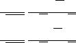
Bode diagrams of the classic fractional integrator of order 0.5 in a finite aluminum
medium are represented in Figure 11. |
|
|
|
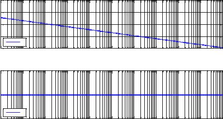
The frequency response study of the function ( |
) allows |
understanding |
the |
influence of the finite character of the medium on the temperature at |
. Actually Figure |
||
12 represents Bode diagrams of this transfer for three different values of |
* |
+ |
|
in a finite aluminum medium. |
|
|
|
Gain (dB)
Phase (deg)
40 |
|
|
|
|
|
|
|
|
|
|
|
0 |
|
|
|
|
|
|
|
|
|
|
|
-40 |
|
|
|
|
|
|
|
|
|
|
|
-80 |
|
|
|
|
|
|
|
|
|
|
|
|
|
0 |
|
|
|
|
|
|
|
|
|
-120 |
-7 |
-6 |
-5 |
-4 |
-3 |
-2 |
-1 |
0 |
1 |
2 |
3 |
10 |
10 |
10 |
10 |
10 |
10 |
10 |
10 |
10 |
10 |
10 |
|
0 |
|
|
|
|
|
|
|
|
|
|
|
-45 |
|
|
|
|
|
|
|
|
|
|
|
|
|
0 |
|
|
|
|
|
|
|
|
|
-90 |
-7 |
-6 |
-5 |
-4 |
-3 |
-2 |
-1 |
0 |
1 |
2 |
3 |
10 |
10 |
10 |
10 |
10 |
10 |
10 |
10 |
10 |
10 |
10 |
|
Frequency (rad/s)
|
|
Figure 11. Bode diagrams of |
( |
) in a finite medium at |
. |
||||||||
Two asymptotic behaviors clearly appear: |
|
|
|
|
|
|
|
||||||
At the low frequencies, a fractional integration behavior of order |
prevails. Actually, |
||||||||||||
|
|
, ( |
) |
. |
|
/ |
|
|
|
|
|
|
|
|
|
|
|
|
|
|
|
|
|
||||
|
|
|
|
{ | |
( |
|
)| |
. |
|
/ |
|
|
(73) |
|
|
|
|
|
|
||||||||
|
|
|
|
|
( ( |
|
)) |
|
|
|
|
|
|
|
|
|
|
|
|
|
|
|
|
|
|||
Complimentary Contributor Copy

112 |
Riad Assaf, Roy Abi Zeid Daou, Xavier Moreau et al. |
|
|
t the |
high frequencies, a proportional |
behavior prevails. Actually, |
|
|
, |
|
|
||||||
( |
) |
|
|
|
|
|
|
{ |
| ( |
)| |
(74) |
||
|
|
( ( |
)) |
|
|
|
The transitional zone between the two asymptotic behaviors is four decades wide and it is centered on the transitional frequency .
Gain (dB)
80 
40 
0
1
10
100
Phase (deg)
10-7 |
10-6 |
10-5 |
10-4 |
10-3 |
10-2 |
10-1 |
100 |
101 |
102 |
103 |
|
45 |
|
|
|
|
|
|
|
|
|
|
|
0 |
|
|
|
|
|
|
|
|
|
|
|
-45 |
|
|
|
|
|
|
|
|
|
|
1 |
|
|
|
|
|
|
|
|
|
|
10 |
|
|
|
|
|
|
|
|
|
|
|
|
|
|
|
|
|
|
|
|
|
|
|
|
100 |
-90 |
-7 |
-6 |
-5 |
-4 |
-3 |
-2 |
-1 |
0 |
1 |
2 |
3 |
10 |
10 |
10 |
10 |
10 |
10 |
10 |
10 |
10 |
10 |
10 |
|
Frequency (rad/s)
Figure 12. Bode diagrams of of ( |
) for |
* |
+ . |
Now it is time to study the influence of each of the three cascading blocks on the global transfer function ( ). For this purpose, for and , Figure 13 visualizes the contribution of each block to the global response in a finite aluminum medium.
Two asymptotic behaviors clearly appear:
At the low frequencies, an integration behavior of order prevails. Actually,
, ( |
) |
|
|
| |
( |
)| |
|
|
|
|
|
||
|
|
|
|
|
|
|
|||||||
|
|
|
|
|
|
|
|
|
|
||||
|
|
|
|
|
|
|
|
|
|
||||
|
|
|
|
|
{ |
( ( |
)) |
|
|
|
|
(75) |
|
|
|
|
|
|
|
|
|
|
|
|
|||
|
|
|
|
|
|
|
|
|
|
|
|||
At the high frequencies, a fractional integration behavior of order |
prevails. Actually, |
||||||||||||
|
|
, ( |
) |
. |
|
/ |
|
|
|
|
|
|
|
|
|
|
|
|
|
|
|
|
|||||
Complimentary Contributor Copy
From the Formal Concept Analysis to the Numerical Simulation … |
113 |
|||||
|
|
|
|
|
|
|
{ | ( |
)| . |
|
/ |
|
|
(76) |
|
||||||
( ( |
)) |
|
|
|
|
|
|
|
|
|
|
||
Here also, the transitional zone between the two asymptotic behaviors is four decades wide and it is centered on the transitional frequency .
Gain (dB)
Phase (deg)
40 
0 


 -40
-40 
-80
-120 |
-7 |
-6 |
-5 |
-4 |
-3 |
-2 |
-1 |
10 |
10 |
10 |
10 |
10 |
10 |
10 |
|
45 |
|
|
|
|
|
|
|
0 |
|
|
|
|
|
|
|
-45 |
|
|
|
|
|
|
|
-90 |
|
|
|
|
|
|
|
-135 |
-7 |
-6 |
-5 |
-4 |
-3 |
-2 |
-1 |
10 |
10 |
10 |
10 |
10 |
10 |
10 |
|
Frequency (rad/s)
H(0,jw,1m)
H0I0.5(0,jw)
F(0,jw,1m)
G(0,jw,1m)
100 101
H(0,jw,1m)
H0I0.5(0,jw)
F(0,jw,1m)
G(0,jw,1m)
100 101
Figure 13. Bode diagrams of ( |
) |
( ) ( |
) and ( |
). |
|
For different values of |
* |
+ |
, (Figure 14 represents the respective Bode |
||
diagrams in a finite aluminum medium illustrating the translation of the transitional zone towards the high frequencies when decreases.
Gain (dB)
Phase (deg)
40 
0
-40
-80
-120  10-7
10-7
0 
-45
-90
-135  10-7
10-7
1
10
100
10-6 10-5 10-4 10-3 10-2 10-1 100 101 102 103
1
10
100
10-6 |
10-5 |
10-4 |
10-3 |
10-2 |
10-1 |
100 |
101 |
102 |
103 |
|
|
|
|
Frequency (rad/s) |
|
|
|
|
|
Figure 14. Bode diagrams of ( |
) for |
* |
+ . |
Complimentary Contributor Copy
114 |
Riad Assaf, Roy Abi Zeid Daou, Xavier Moreau et al. |
|
|
For different values of * + , Figure 15 represents respectively ( ) in Black-Nichols plane in a finite aluminum medium.
6.4. Frequency Behavior Analysis for
|
For |
, |
( |
) |
. Thus it is interesting |
to begin with the study |
of its |
||||||||||||
frequency behavior in order to understand its influence on the global response ( |
). |
||||||||||||||||||
(Eq. 56-59) reformulate the expression of the third block: |
|
|
|
|
|||||||||||||||
|
|
|
|
|
|
|
|
|
|
|
|
|
|
|
|
|
|
|
|
|
|
|
|
|
( |
)√ ⁄ |
( |
|
)√ ⁄ |
|
|
|
|
||||||
|
|
|
|
( |
) |
|
|
|
|
|
|
|
|
|
|
|
|
|
(77) |
|
|
|
|
|
|
|
|
|
|
|
|
|
|
|
|
|
|||
|
|
|
|
√ ⁄ |
|
|
√ ⁄ |
|
|
|
|||||||||
|
|
|
|
|
|
|
|
|
|
|
|
|
|||||||
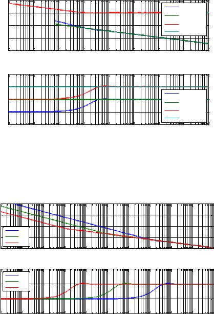
|
Figure 16 represents Bode diagrams of the transfer of |
( |
) for a finite aluminum |
||||||||||||||||
medium of length |
|
|
and for four different values |
|
of the temperature sensor position, |
||||||||||||||
let |
* |
+ |
. |
|
|
|
|
|
|
|
|
|
|
|
|
|
|
|
|
|
Two behaviors clearly appear: |
|
|
|
|
|
|
|
|
|
|
|
|
|
|
|
|||
|
At the low frequencies, |
|
|
|
|
|
|
|
|
|
|
|
|
|
|
|
|
||
|
|
|
|
( |
) |
|
{ |
|
| ( |
( |
|
|
|
|
)| |
(78) |
|||
|
|
|
|
|
|
|
|
|
|
( |
|
|
|
|
)) |
|
|||
Gain (dB)
40
1
20 |
|
10 |
|
||
|
|
100
0
-20
-40
-60
-80
-100
-120 |
|
|
|
|
|
|
|
-270 |
-225 |
-180 |
-135 |
-90 |
-45 |
0 |
45 |
Phase (deg)
Figure 15. Black-Nichols plots of ( |
) for |
* |
+ |
Complimentary Contributor Copy
From the Formal Concept Analysis to the Numerical Simulation … |
115 |
|
|
Gain (dB)
Phase (deg)
40 |
|
|
|
|
|
|
|
|
0 |
|
|
|
|
|
|
|
|
-40 |
|
50 |
|
|
|
|
|
|
|
|
|
|
|
|
|
|
|
|
|
10 |
|
|
|
|
|
|
-80 |
|
5 |
|
|
|
|
|
|
|
|
0 |
|
|
|
|
|
|
-120 |
-5 |
-4 |
-3 |
-2 |
-1 |
0 |
1 |
2 |
10 |
10 |
10 |
10 |
10 |
10 |
10 |
10 |
|
45 |
|
|
|
|
|
|
|
|
0 |
|
|
|
|
|
|
|
|
-45 |
|
50 |
|
|
|
|
|
|
|
|
|
|
|
|
|
|
|
|
|
10 |
|
|
|
|
|
|
-90 |
|
5 |
|
|
|
|
|
|
|
|
0 |
|
|
|
|
|
|
-135 |
-5 |
-4 |
-3 |
-2 |
-1 |
0 |
1 |
2 |
10 |
10 |
10 |
10 |
10 |
10 |
10 |
10 |
|
Frequency (rad/s)
Figure 16. Bode diagrams of |
( |
|
) for |
* |
|
|
+ |
. |
|||||||
At the high frequencies, |
|
|
|
|
|
|
|
|
|
|
|
|
|
|
|
|
|
|
|
|
|
| |
( |
|
)| |
. |
|
|
/ |
|
|
( |
) |
√ |
|
{ |
|
(79) |
|||||||||
|
|
|
|
||||||||||||
|
|
|
|
|
|
||||||||||
|
|
|
|
|
|||||||||||
|
|
|
|
|
|
|
|
|
|
|
|
||||
|
|
|
|
|
|
( |
( |
|
)) |
. |
|
|
/ |
||
|
|
|
|
|
|
|
|
||||||||
In order to make the analysis easier, a special frequency |
|
is introduced; it is defined as: |
|||||||||||||
|
|
|
|
|
|
|
|
|
|
|
|
|
|||
|
|
| ( |
|
|
)| |
⁄√ |
|
|
|
|
|
|
|
(80) |
|
The frequency |
decreases when |
increases. This is why, for a given frequency , the |
|||||||||||||
gain and the phase are as smaller as is big as it is evident in Figure 16.
Now it is time to study the influence of each of the four cascading blocks on the global transfer function ( ). For this purpose, for and , Figure 17 visualizes the contribution of each block to the global response in a finite aluminum medium.
Three behaviors clearly appear:
At the low frequencies, an integration behavior of order prevails similar to the one
found at |
. Actually, |
|
, ( |
) |
|
|
|
|
|
|
|
|
|
||||||||
|
| ( |
|
)| |
|
|
|
|
|
|
|
|
|
|
|
|
|
|
|
|||
|
{ |
|
|
(81) |
||||||
|
( |
( |
)) |
|
|
|
|
|
|
|
|
|
|
|
|
|
|
||||
Complimentary Contributor Copy

116 |
Riad Assaf, Roy Abi Zeid Daou, Xavier Moreau et al. |
|
|
Gain (dB)
Phase (deg)
40 |
|
|
|
|
|
|
|
|
|
|
0 |
|
|
|
|
|
|
|
|
|
|
|
|
|
|
|
|
H(5mm,jw,1m) |
|
|
|
|
-40 |
|
|
|
|
|
H I0.5(0,jw) |
|
|
|
|
|
|
|
|
|
|
0 |
|
|
|
|
-80 |
|
|
|
|
|
F(0,jw,1m) |
|
|
|
|
|
|
|
|
|
|
G(5mm,jw,1m) |
|
|
|
|
-120 |
-7 |
-6 |
-5 |
-4 |
-3 |
-2 |
-1 |
0 |
1 |
2 |
10 |
10 |
10 |
10 |
10 |
10 |
10 |
10 |
10 |
10 |
|
45 |
|
|
|
|
|
|
|
|
|
|
0 |
|
|
|
|
|
|
|
|
|
|
-45 |
|
|
|
|
|
|
|
|
|
|
-90 |
|
|
|
|
|
|
|
|
|
|
-135 |
|
|
|
|
|
|
|
|
|
|
10-7 |
10-6 |
10-5 |
10-4 |
10-3 |
10-2 |
10-1 |
100 |
101 |
102 |
|
|
|
|
|
|
Frequency (rad/s) |
|
|
|
|
|
|
Figure 17. Bode diagrams of |
( |
) |
( ) |
( |
) and |
( |
). |
At the medium frequencies, a |
fractional |
integration |
behavior of |
order |
prevails. |
|||
Actually, |
, ( |
) |
( |
) |
|
|
|
|
|
|
|
|
{ | |
( |
)| |
. |
|
|
/ |
|
|
|
|
|
|
|
(82) |
|||
|
|
|
|
|
|
|
|
|
|
|
|
||||||||||
|
|
|
|
|
( |
( |
)) |
|
|
|
|
|
|
|
|
|
|
|
|
|
|
|
|
|
|
|
|
|
|
|
|
|
|
|
|
|
|
|
|||||
|
At the high frequencies, a behavior identical to the one in the semi-infinite medium |
||||||||||||||||||||
|
|
|
|
|
|
|
|
|
|
|
|
|
|
|
|
|
|
|
|||
prevails. Actually, |
, |
( |
) |
|
( |
|
|
) |
|
|
√ |
|
|
|
|||||||
|
|
|
|
|
|
|
|||||||||||||||
|
|
|
{ |
| ( |
|
)| . |
|
/ |
|
|
|
|
. |
|
|
/ |
|
|
(83) |
||
|
|
|
|
|
|
|
|
|
|
|
|
|
|||||||||
|
|
|
|
|
|
|
|
|
|
|
|
|
|
|
|
|
|||||
|
|
|
|
|
|
|
|
|
|
|
|
|
|
|
|
||||||
|
|
|
|
|
|
|
|
|
|
|
|
|
|
|
|
|
|
|
|
||
|
|
|
|
( ( |
|
)) |
|
|
|
|
|
|
. |
|
/ |
|
|
||||
|
|
|
|
|
|
|
|
|
|
|
|
|
|
||||||||
|
Figure 18 represents Bode diagrams of the transfer of |
( |
|
|
) for a finite aluminum |
||||||||||||||||
medium of length |
and for four different values |
of the temperature sensor position, |
|||||||||||||||||||
let |
* |
+ |
. |
|
|
|
|
|
|
|
|
|
|
|
|
|
|
|
|
|
|
|
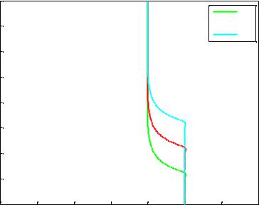
For a finite aluminum medium of length |
|
|
|
|
and for four different values of the |
|||||||||||||||
temperature |
sensor |
position, |
let |
* |
|
+ |
|
|
, |
Figure 19 |
represents respectively |
||||||||||
( |
) in Black-Nichols plane. |
|
|
|
|
|
|
|
|
|
|
|
|
|
|
|
|
|
|||
Complimentary Contributor Copy