130 |
Fady Christophy, Xavier Moreau, Roy Abi Zeid Daou et al. |
|
|
the expression of order 0.5 could be interpreted as a closed loop system (figure 5), the open loop transfer function is equal to the product of a constant x0.5 and a fractional integrator I0.5(s), the latter having already been subjected to the approximation described above.
|
|
E x, s |
T 0, s |
+ |
T x, s |
|
|
- |
Figure 5. Block diagram associated with the approximation of the function E(x,s).
In summary, obtaining the rational model for temporal simulation, x 0 , is due to the rational integrator I N0.5 s whose center frequency m is chosen equal to the crossover
frequency, unom, in nominal open loop.
Figure 6 shows the block diagram of the rational model used in Simulink for time response simulation.
|
|
|
|
|
|
|
|
|
|
|
T 0,0 |
|
|
|
|
|
|
T x,0 |
|
|
|
|
|
|
t |
|
|
|
0.5 |
|
|
|
T 0,t |
|
|
|
|
|
|
|
|
u t f t |
|
|
|
|
|
|
T |
0, t |
|
+ |
|
|
|
|
|
|
+ |
T x, t |
||
|
|
|
|
|
|
|
|
|
|
|
|
|
||||||||
|
|
|
|
|
|
|
||||||||||||||
|
|
|
|
|
|
|
|
|
|
|
+ |
- |
|
|
|
|
|
|
||
|
|
|
|
|
|
|
|
|
|
|
|
|
|
|
|
|
||||
|
|
|
|
|
|
|
|
|
|
|
|
|
|
|
|
|
|
|
||
|
|
|
|
|
|
|
|
|
|
|
|
|
|
|
|
|
|
|
|
|
|
|
|
|
|
|
|
|
|
|
|
|
|
|
|
|
|
|
|
|
|
|
|
|
|
|
|
|
|
|
|
|
|
|
|
|
|
|
|
|
|
|
|
|
|
|
|
|
|
|
|
|
|
|
|
|
|
|
|
|
|
|
|
Figure 1. Block diagram of the rational model used in Simulink for time response simulation.
Remark. In a second step, an optimal approach to managing the dilemma between the fidelity of the approximation which may be improved by increasing the order K of the truncation of the series (16) (by increasing the complexity), and the simulation time which unfortunately also increases with the degree of complexity is proposed. A fractional representation of order 0.5 is studied in particular for the formulation of the optimal approach, the value of the order K directly fixing the number of fractional integrators. Similarly, the optimum choice of the number of decades and cells in the synthesis of rational integrator will be a specific study.
Finally, the approximation errors of the rational model may be considered as uncertainties and used for the control-system design.
3. Temperature Control
3.1. Scheme for the Control-System Design
Figure 7 shows the scheme used for the control-system design.
Complimentary Contributor Copy

Temperature Control of a Diffusive Medium Using the CRONE Approach |
131 |
||||||||||||
|
|
|
|
|
|
|
|
|
|
|
|
||
|
|
|
|
Input disturbance |
|
Sensor noise |
|
||||||
|
|
|
|
|
|
Du(s) |
|
|
Dm(s) |
|
|||
|
Error signal |
|
|
|
|
|
|
|
|
||||
Yref(s) + |
|
|
(s) |
|
|
U(s) |
|
|
|
|
|
Y(s) |
|
|
|
|
|
|
|
|
|
||||||
Reference |
- |
|
C(s) |
|
+ |
|
G(s) |
|
+ |
|
Measured |
|
|
|
|
|
|
|
|
||||||||
|
|
|
|
|
|
|
|
|
|
||||
signal |
Controller |
Plant model |
|
|
|
||||||||
|
|
|
|
output |
|
||||||||
|
|
|
|
|
|
||||||||
|
|
|
|
|
|
|
|
|
|
|
|
|
|
|
|
|
|
|
|
|
|
|
|
|
|
|
|
Figure 7. Scheme used for the control-system design.
The equations associated with the scheme of figure 7 are: for the output signal:
Y s S s Dm s S s G s Du s T s Yref s ; |
(18) |
|||||
for the error signal: |
|
|
|
|
|
|
s S s Dm s S s G s Du s S s Yref s ; |
(19) |
|||||
for the control signal: |
|
|
|
|
|
|
U s S s C s Dm s T s Du s S s C s Yref s , |
(20) |
|||||
with |
|
|
|
|
|
|
S s |
1 |
|
|
: |
Sensitivity function |
|
1 s |
|
|||||
|
|
|
|
|||
T s 1 S |
s : |
|
Complementary sensitivity function . |
(21) |
||
|
|
|
|
|
|
|
s C s G s : Open loop transfer function
3.2. Summary Data
The required data for the control-system design are divided into two groups:
Signals models (often difficult to obtain, especially regarding the measurement noise) and the uncertain especially linear model of the process which in the case of a frequency approach is in the form of a transfer function G(s) (Figure 7), the areas of
uncertainty parameters i are specified, for example, in the form of bounded intervals, i i ; i ;
Translating specifications:
Complimentary Contributor Copy
132 |
Fady Christophy, Xavier Moreau, Roy Abi Zeid Daou et al. |
|
|
o Degree of stability, through the stability margins, M , MG, MM;
o Speed, through the unit gain frequency in open loop, u u min ; u max ;
o Accuracy in the steady state, through the relative error, (%); o Saturation, through the maximum value of the command, Umax.
Remark. It should be noted that the translation of specifications requires preliminary work, especially regarding the choice of u.
In the absence of additional information, particularly regarding the measurement noise, it is difficult (or impossible) to determine precisely unom.
However, a simplified approach leading to a first iteration can be made by taking unom
= 3 0nom, initial choice based on experience…
Another approach is to set the contribution cm of measurement noise relative to the maximum value Umax of control signal (for instance cm = 10%). In the absence of precise model of the measurement noise, knowing that its frequency spectrum is more concentrated towards the high frequencies, we place ourselves in stationary harmonic, we estimate the amplitude Dm of measurement noise over the full scale range Em of the sensor (for instance Dm = 1% Em) and from equation (3) we impose:
|
|
lim |
|
|
U j |
|
|
|
lim |
|
S j C j |
|
Dm cm Umax , |
(22) |
|||||||
|
|
|
|
|
|||||||||||||||||
|
|
|
|
|
|
|
|
|
|
|
|
|
|
|
|
||||||
|
|
|
|
|
|
|
|
|
|
|
|
|
|
|
|||||||
knowing that lim |
|
S j |
|
1, |
|
|
|
|
|
|
|
|
|
|
|
|
|
||||
|
|
|
|
|
|
|
|
|
|
|
|
|
|
|
|||||||
|
|
lim |
|
U j |
|
lim |
|
C j |
|
Dm cm Umax . |
(23) |
||||||||||
|
|
|
|
|
|
||||||||||||||||
|
|
|
|
|
|
||||||||||||||||
|
|
|
|
|
|
|
|
|
|
|
|
|
|
||||||||
|
|
|
|
|
|
|
|
|
|
|
|
|
|
|
|||||||
Thus, a strain is obtained regarding the controller gain at high frequencies:
C lim |
|
C j |
|
|
cm Umax |
, |
(24) |
|
|
|
|||||||
|
|
|
||||||
|
|
|
|
|
|
Dm |
|
|
|
|
|
|
|
|
|||
constraint leads to limit u.
3.3. Loop Shaping
There are three generations of the CRONE controller [Oustaloup, 1995]. When parametric uncertainties result in gain variations in open loop, the second generation is used. Hence, the expression of the open loop transfer function (s) is given by:
|
|
|
1 s / |
l |
nl |
1 s / |
h |
n |
1 s / |
|
nh , |
|
|
(s) |
|
|
|
|
|
|
|
|
(25) |
||||
0 |
|
|
|
|
h |
||||||||
|
|
s / l |
|
|
|
|
|
|
|
|
|
||
|
|
|
|
|
1 s / l |
|
|
|
|
||||
where ωl and ωh represent the transitional low and high frequencies, n the non-integer order between 1 and 2 near the frequency ωu, nl and nh are the orders of the asymptotic behavior at
Complimentary Contributor Copy

Temperature Control of a Diffusive Medium Using the CRONE Approach |
133 |
|
|
low and high frequencies (figure 8) and β0 a constant which ensures unity gain at frequency ωu. β0 is given by:
|
0 |
|
/ |
nl |
1 |
/ |
2 n nl / 2 1 |
/ |
h |
2 |
nh n / 2 . |
(26) |
|
u |
l |
|
u |
l |
u |
|
|
|
|
The fractional asymptotic behavior (figure 8) is set to a frequency interval [ωA, ωB] around the nominal frequency ωunom. To meet the robustness of the degree of stability, it is necessary to impose:
u u min ; u max , A u B |
|
|
|
|
|
|
A |
u min . |
|
|
|
|
B |
|
|
|
|
u max |
Open-loop gain
Log10( h)
0 dB |
|
|
|
|
|
|
Log10( B) |
|
|
|
|
|
|
Log10( unom) |
|
|
|
|
|
Log10( A) |
|||
|
|
|
|
|
|
||
|
|
|
|
|
|
|
|
|
|
|
Log10( l) |
|
|
|
|
|
|
|
|
|
|
|
|
Openloop- |
phase |
|
|
|
Fractional asymptotic behavior |
||
|
|
|
|
|
|
|
|
|
10 |
|
10 |
||||
0 ° |
|
|
|
|
|
|
|
-n l 90 °
-n 90 °
-n h 90 °
Figure 8. Asymptotic Bode diagrams of (j ).
(27)
Log10( )
Log10( )
In addition, to obtain a fractional asymptotic behavior on the interval [ωA, ωB] (Figure 8), a practical rule leads to choose [Oustaloup, 1995]
|
|
|
/10 |
. |
(28) |
||
|
l |
|
A |
|
|
||
|
10 |
B |
|
|
|||
|
h |
|
|
|
|
|
|
Complimentary Contributor Copy

134 Fady Christophy, Xavier Moreau, Roy Abi Zeid Daou et al.
Taking l and h geometrically distributed around unom and introducing a = B/ A:
l and h are given by:
l h
hl
|
l h |
unom |
|
|
|
|||
|
|
|
|
|||||
|
|
B |
|
, |
|
|
|
|
a |
|
|
|
|
|
|
|
|
A |
|
|
|
|
|
|||
|
|
|
|
|
|
|
||
unom |
|
|
|
|
/ 10 |
a |
|
|
|
|
|
|
. |
||||
|
|
l |
unom |
|
|
|||
|
|
|
|
|
|
10 |
a |
|
|
|
|
|
h |
unom |
|
|
|
(29)
(30)
20 Log10 0 dB |
|
|
|
Log10 |
|
|
|
Log10 B |
|
Log10 A |
Log |
10 |
|
|
|
|
unom |
|
Log10 B - Log10 A = Log10( B/ A)
= Log10a
Figure 9. Illustration of computing a.
As for the calculation of the ratio a, it is derived from the slope of –n20dB/dec near unom and the gain variation in open loop due to parametric uncertainties (figure 9). Thus, we find out:
a 1/ n . |
(31) |
Finally, given that
(s) Ccrone s G s , |
(32) |
the fractional form CF(s) of the transfer function of the CRONE regulator Ccrone(s) is deducted from the transfer function Gnom(s) of the nominal process:
CF s (s) / Gnom s . |
(33) |
Finally, one last step is necessary to determine the rational form CR(s) of the fractional transfer function CF(s) which is obtained either analytically using a recursive distribution of poles and zeros [Oustaloup, 1995], either numerically from the frequency response of CF(j ) and a specific module of the CRONE Toolbox [Oustaloup, 2005].
Complimentary Contributor Copy
Temperature Control of a Diffusive Medium Using the CRONE Approach |
135 |
|
|
Remark. Be careful, if the process is non minimum phase (positive real part zeros) and if it has a delay and / or very little damped modes, then there are precautions to take [Oustaloup, 2005].
3.4. Specifications and Results
Finally, the translation of specifications led to choose:
o for the degree of stability, phase margin M 45;
o for the speed, crossover frequency, unom, in nominal open loop the greatest possible; o for accuracy in the steady state, a static error equal to zero;
o to saturation, a maximum value of the control signal, Umax = 12 W.
Given the summary data, we choose:
nl = 1.5, to ensure zero steady-state error;
n = (180° - M )/90° = 1.5, to ensure a phase margin M = 45;
nh = 1.5, to limit the input sensitivity;
unom = 30nom = 0.53 rad/s (simplified approach).
From these data and taking into consideration the relation (31), we deduce:
a 2.171/1.5 1.68 |
|
|
|
|
0.41 rad/s |
|
|
0.041 rad/s |
. |
(34) |
|
A |
u min |
0.684 rad/s |
l |
6.84 rad/s |
|||||
|
|
|
B |
|
|
|
|
|
||
|
|
|
u max |
|
|
h |
|
|
|
The expression of the transfer function is given by:
|
|
|
1 s / l |
1.5 |
|
1 s / h |
1.5 |
|
|
1.5 |
|
|
(s) |
0 |
|
|
|
|
|
|
1 s / |
h |
|
, |
(35) |
|
|
|||||||||||
|
|
s / l |
|
|
1 s / l |
|
|
|
|
|
||
|
|
|
|
|
|
|
|
|
|
|
||
with |
|
|
|
|
|
|
|
|
|
|
|
|
|
|
|
|
0 |
46.6 . |
|
|
|
|
|
(36) |
|
From the relations (32) and (33), we deduce the expression of the fractional form CF(s) of the CRONE regulator:
|
|
|
|
|
1 s / |
l |
1.5 |
|
1 s / |
h |
C |
|
(s) |
|
|
|
|
|
|
||
F |
0 |
|
|
|
|
|||||
|
|
|
s / l |
|
|
|
1 s / l |
|||
|
|
|
|
|
|
|
|
|||
1.5
1 s / |
1.5 |
|
s 0.5 |
|
(37) |
|
h |
|
|
|
, |
||
|
|
|
|
|
|
|
|
|
|
1nom |
|
|
|
after simplification,
Complimentary Contributor Copy

136 |
Fady Christophy, Xavier Moreau, Roy Abi Zeid Daou et al. |
|
|
|
|
|
|
C |
|
(s) |
C0 |
, |
(38) |
||
|
|
|
|
F |
s |
||||||
|
|
|
|
|
|
|
|
|
|||
|
|
|
|
|
|
|
|
|
|
||
with |
|
|
|
|
|
|
|
|
|
|
|
|
|
|
1.5 |
|
|
|
|
|
|
|
|
C |
|
|
l |
|
|
C 9.14510 1 W / K . |
(39) |
||||
0 |
|
0.5 |
|
||||||||
0 |
|
|
0 |
|
|
||||||
|
|
|
1nom |
|
|
|
|
|
|
||
Remark. The nature of the plant (integrator of order 0.5) and the choice of orders asymptotic behavior at low (nl = 1.5), at average (n = 1.5) and at high (nh = 1.5) frequencies lead to a particular case where the expression CF(s) is already in a very simple rational form (an integrator of order 1). In fact, for this particular case, the transfer function (s) in open loop is an integrator of order 1.5:
|
|
1.5 |
(40) |
(s) |
u . |
||
|
s |
|
|
Sensitivity function S(s) and complementary sensitivity function T(s) have the following expressions:
|
|
S(s) |
|
1 |
|
s / u 1.5 |
|
|
(41) |
|
|
1 (s) |
1 s / u 1.5 |
|
|||||
and |
|
|
|
|
|
|
|
|
|
|
|
T (s) |
(s) |
|
1 |
|
|
|
|
|
|
1 (s) |
1 s / u 1.5 . |
|
(42) |
||||
(dB) |
40 |
|
|
|
|
|
|
Alu. |
|
Gain |
|
|
|
|
|
|
|
||
|
|
|
|
|
|
|
|
||
20 |
|
|
|
|
|
|
Cop. |
|
|
|
|
|
|
|
|
|
|
||
loop |
0 |
|
|
|
|
|
|
Iron |
|
-20 |
|
|
|
|
|
|
|
|
|
Open- |
|
|
|
|
|
|
|
|
|
-40 |
-2 |
10 |
-1 |
|
10 |
0 |
10 |
1 |
|
|
10 |
|
|
|
|
|
|||
(deg.) |
|
|
|
Frequency (rad/s) |
|
|
|
||
0 |
|
|
|
|
|
|
|
|
|
|
|
|
|
|
|
|
|
|
|
Phase |
-45 |
|
|
|
|
|
|
|
|
-90 |
|
|
|
|
|
|
|
|
|
loop |
-135 |
|
|
|
|
|
|
|
|
Open- |
10-2 |
10-1 |
|
100 |
101 |
||||
|
-180 |
|
|
|
|
|
|
|
|
|
|
|
|
Frequency (rad/s) |
|
|
|
||
Figure 10. Bode diagrams of (j ).
Complimentary Contributor Copy

Temperature Control of a Diffusive Medium Using the CRONE Approach |
137 |
|
|
3.4.1. Frequency Responses at x = 0
Figures 10 and 11 show Bode diagrams and Black-Nichols diagrams of the transfer function in open loop (s) for the nominal parametric state, and for the extreme values of gain. The robustness of the degree of stability is ensured, due to the insensitivity of the phase margin M to parametric uncertainties.
|
40 |
|
|
|
|
|
|
|
|
|
|
|
0 dB |
|
|
|
30 |
|
|
|
|
|
|
(dB) |
20 |
1 dB |
|
|
|
|
|
10 |
3 dB |
|
|
|
|
|
|
Gain |
|
|
|
|
|
||
|
6 dB |
|
|
|
|
|
|
|
|
|
|
|
|
|
|
loop |
0 |
|
|
|
|
|
|
|
|
|
|
|
|
|
|
Open- |
-10 |
|
|
|
|
|
|
-20 |
|
|
|
|
|
|
|
|
|
|
|
|
|
|
|
|
-30 |
|
|
|
|
|
|
|
-40 |
|
|
|
|
|
|
|
-270 |
-225 |
-180 |
-135 |
-90 |
-45 |
0 |
|
|
|
Open-loop Phase (deg.) |
|
|
||
Figure 11. Black-Nichols diagram of (j ).
|
5 |
|
|
|
|
|
|
|
|
0 |
|
|
|
|
|
|
|
|
-5 |
|
|
|
|
|
|
|
|
-10 |
|
|
|
|
|
|
|
(dB) |
-15 |
|
|
|
|
|
|
|
|
|
|
|
|
|
|
|
|
Gain |
-20 |
|
|
|
|
|
|
|
|
|
|
|
|
|
|
|
|
|
-25 |
|
Alu. |
|
|
|
|
|
|
|
|
|
|
|
|
|
|
|
-30 |
|
Cop. |
|
|
|
|
|
|
|
Iron |
|
|
|
|
|
|
|
|
|
|
|
|
|
|
|
|
-35 |
|
|
|
|
|
|
|
|
-40 |
-2 |
10 |
-1 |
10 |
0 |
10 |
1 |
|
10 |
|
|
|
|
|||
|
|
|
|
Frequency (rad/s) |
|
|
|
|
Figure 12. Gain diagram of the complementary sensitivity function T(s).
Complimentary Contributor Copy

138 |
Fady Christophy, Xavier Moreau, Roy Abi Zeid Daou et al. |
|
|
Figures 12 and 13 show diagrams of the complementary sensitivity function T(s) (figure 12) and the sensibility function S(s) (figure 13) for the nominal parametric state, and for the extreme values of the uncertainties. The robustness of the degree of stability appears with insensitivity of the resonance factors T(j ) et S(j ) to parametric uncertainties.
Figure 14 shows diagrams of the sensitivity function input R(s) = S(s)C(s). We can notice that the gains R(j ) are maximum at medium frequencies.
|
5 |
|
|
|
|
|
|
|
|
0 |
|
|
|
|
|
|
|
|
-5 |
|
|
|
|
|
|
|
|
-10 |
|
|
|
|
|
|
|
(dB) |
-15 |
|
|
|
|
|
|
|
|
|
|
|
|
|
|
|
|
Gain |
-20 |
|
|
|
|
|
|
|
|
|
|
|
|
|
|
|
|
|
-25 |
|
|
|
|
|
|
|
|
-30 |
|
|
|
|
|
Alu. |
|
|
|
|
|
|
|
Cop. |
|
|
|
|
|
|
|
|
|
|
|
|
-35 |
|
|
|
|
|
Iron |
|
|
|
|
|
|
|
|
|
|
|
-40 |
-2 |
10 |
-1 |
10 |
0 |
10 |
1 |
|
10 |
|
|
|
|
|||
|
|
|
|
Frequency (rad/s) |
|
|
|
|
Figure 13. Gain diagram of the sensibility function S(s).
|
10 |
|
|
|
|
|
|
|
|
|
|
|
|
|
|
Alu. |
|
|
5 |
|
|
|
|
|
Cop. |
|
|
|
|
|
|
|
Iron |
|
|
|
|
|
|
|
|
|
|
|
|
0 |
|
|
|
|
|
|
|
(dB) |
-5 |
|
|
|
|
|
|
|
Gain |
|
|
|
|
|
|
|
|
|
|
|
|
|
|
|
|
|
|
-10 |
|
|
|
|
|
|
|
|
-15 |
|
|
|
|
|
|
|
|
-20 |
-2 |
10 |
-1 |
10 |
0 |
10 |
1 |
|
10 |
|
|
|
|
|||
|
|
|
|
Frequency (rad/s) |
|
|
|
|
Figure 14. Gain diagram of the sensitivity function of the input R(s)= S(s)C(s).
Complimentary Contributor Copy
Temperature Control of a Diffusive Medium Using the CRONE Approach |
139 |
|
|
3.4.2. Time Responses at x = 0
The rational model of the process used for the time simulation is derived from the rational integrator I N0.5 s (relation (13)) obtained by taking a median frequency m = unom =
0.53 rad/s, a constant A = b/a = 108 (an approximation of 8 decades) and a number of cells N = 20.
Figure 15 shows, at x = 0 and for aluminum, the step responses of the temperature to a flux of amplitude 1 W obtained from the exact response (relation (3)) and the response of the approximated model.
|
3.5 |
|
|
|
|
|
|
3 |
|
|
|
|
|
(°C) |
2.5 |
|
|
|
|
|
|
|
|
|
|
|
|
Temperature |
2 |
|
|
|
|
|
1.5 |
|
|
|
|
|
|
|
|
|
|
|
|
|
|
1 |
|
|
|
|
|
|
0.5 |
|
|
|
Alu. x=0 exact. |
|
|
|
|
|
|
|
|
|
|
|
|
|
Alu. x=0 approxim. |
|
|
00 |
10 |
20 |
30 |
40 |
50 |
Time (s)
Figure 15. Step responses of the temperature at a flux of amplitude 1 W, at x = 0, for aluminum, obtained from the exact response (relation (3)) and the response of the approximated model.
|
0.5 x 10⁻³ |
|
|
|
|
|
|
0 |
|
|
|
|
|
(°C) |
-0.5 |
|
|
|
|
|
difference |
|
|
|
|
|
|
-1 |
|
|
|
|
|
|
|
|
|
|
|
|
|
Temperature |
-1.5 |
|
|
|
|
|
-2 |
|
|
|
|
|
|
|
|
|
|
|
|
|
|
-2.5 |
|
|
|
|
|
|
-30 |
10 |
20 |
30 |
40 |
50 |
Time (s)
Figure 16. Temperature difference, at x = 0 and for aluminum, between the exact step response (relation (3)) and the approximated model.
Complimentary Contributor Copy

140 |
Fady Christophy, Xavier Moreau, Roy Abi Zeid Daou et al. |
|
|
Figure 16 shows, always at x = 0 and for aluminum, the temperature difference between the exact step response and the approximated model, to assess the quality of the approximation since the maximum error in 50 seconds is less than 3/1000 of °C.
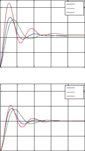
Figure 17 shows the step responses of the output at a step input of amplitude 1°C for the nominal parametric state, and for the extreme values of the uncertainties. The robustness of the degree of stability clearly appears with the insensitivity of the first overshoot and the damping factor.
|
1.4 |
|
|
|
|
|
|
|
|
|
|
|
Alu. |
|
1.2 |
|
|
|
|
Cop. |
|
|
|
|
|
|
|
|
|
|
|
|
|
Iron |
(°C) |
1 |
|
|
|
|
|
|
|
|
|
|
|
|
T(0,t) |
0.8 |
|
|
|
|
|
|
|
|
|
|
|
|
Temperature |
0.6 |
|
|
|
|
|
0.4 |
|
|
|
|
|
|
|
|
|
|
|
|
|
|
0.2 |
|
|
|
|
|
|
00 |
10 |
20 |
30 |
40 |
50 |
Time (s)
Figure 17. Step responses of the output to an input step of 1°C: for aluminum (________), copper (________) and iron (________).
|
1 |
|
|
|
|
|
|
|
|
|
|
Alu. x=0 |
|
|
0.8 |
|
|
|
Cop. x=0 |
|
|
|
|
|
|
|
|
|
|
|
|
|
Iron x=0 |
|
|
0.6 |
|
|
|
|
|
Error (°C) |
0.4 |
|
|
|
|
|
0.2 |
|
|
|
|
|
|
|
0 |
|
|
|
|
|
|
-0.2 |
|
|
|
|
|
|
-0.40 |
10 |
20 |
30 |
40 |
50 |
Time (s)
Figure 18. Step responses of the error to a step input of 1°C: for aluminum (________), copper (________) and
iron (________).
Complimentary Contributor Copy
Temperature Control of a Diffusive Medium Using the CRONE Approach |
141 |
|
|
Figure 18 shows the step responses of the error for the same simulation conditions. According to specifications, the static error is zero.
Finally, figure 19 shows the corresponding step responses of the control signal where the maximum value Umax = 12 W is never reached.
|
2 |
|
|
|
|
|
|
1.8 |
|
|
|
Alu. x=0 |
|
|
|
|
|
Cop. x=0 |
|
|
|
|
|
|
|
|
|
|
1.6 |
|
|
|
Iron x=0 |
|
|
|
|
|
|
|
|
(W) |
1.4 |
|
|
|
|
|
1.2 |
|
|
|
|
|
|
signal |
|
|
|
|
|
|
1 |
|
|
|
|
|
|
Control |
0.8 |
|
|
|
|
|
0.6 |
|
|
|
|
|
|
|
|
|
|
|
|
|
|
0.4 |
|
|
|
|
|
|
0.2 |
|
|
|
|
|
|
00 |
10 |
20 |
30 |
40 |
50 |
Time (s)
Figure 19. Step responses of the control signal to a step input of 1°C: for aluminum (________), copper (________) and iron (________).
3.4.3. Frequency Responses at x > 0
The objective is always to control the temperature T(0,t) at x = 0, but by analyzing the influence of the position x of the temperature sensor when it can’t be positioned at x = 0.
Thus, the transfer function of open loop (x,s) is then given by:
|
|
s 0.5 |
|
|
|
|
|
|
|
|
|
|
|
|
|
||
x, s C s G 0, s |
|
|
|
|
|
e |
x |
, |
(43) |
||
|
|
|
|
|
|
by introducing the nominal transfer function of the open loop nom(0,s),
|
|
|
|
|
s |
0.5 |
|
|
|
|
|
|
|
|
|
|
|
|
|
|
|
||
x, s |
|
0, s |
|
|
|
|
|
nom |
e |
|
x , |
(44) |
|||
|
|
|
|
|
|
|
|
whose frequency response (x,j ) is expressed by:
|
|
|
|
0.5 |
|
|
|
|
|
j |
|
|
|
|
|
|
|
|
||
x, j |
|
0, j e |
|
|
|
|
nom |
|
x . |
(45) |
|||
|
|
|
|
|
|
|
Complimentary Contributor Copy

142 |
Fady Christophy, Xavier Moreau, Roy Abi Zeid Daou et al. |
|
|
Knowing that
|
|
|
0.5 |
|
|
|
|
|
|
|
|
|
|
|
|
|
|
0.5 |
|
|
0.5 |
|
|||||||
|
|
|
|
|
|
|
|
|
|
|
|
|
|
|
|
|
|
|
|
|
|
|
|
|
|
|
|
||
|
|
|
|
|
|
|
|
|
|
|
|
|
|
|
|
|
|
|
x |
|
|
|
|
||||||
|
|
|
|
|
|
|
|
|
|
|
|
|
|
|
|
|
|
|
|
|
|||||||||
j |
|
|
|
|
|
|
|
|
|
|
|
|
|
e |
|
2 x |
|
e |
2 |
|
|
||||||||
|
|
|
m x, |
|
e j x, |
|
|
|
m x, |
|
|
|
|
|
|
|
|
|
|
|
|
||||||||
e |
x |
|
|
|
avec |
|
|
|
|
|
|
|
|
|
0.5 |
|
|
|
|
|
0.5 , |
||||||||
|
|
|
|
|
|
|
|
|
|
|
|
|
|
|
|
|
|
|
|
|
|
||||||||
|
|
|
|
|
|
|
|
|
|
|
x, |
|
|
|
|
|
|
|
x |
|
|
|
|
||||||
|
|
|
|
|
|
|
|
|
|
|
|
|
|
|
|
|
|
|
|||||||||||
|
|
|
|
|
|
|
|
|
|
|
|
|
|
|
|
|
|
|
|
|
|
|
|
2 |
|
||||
|
|
|
|
|
|
|
|
|
|
|
|
|
|
|
|
2 x |
|
|
|
|
|
||||||||
the gain and the argument of the open loop are given by: |
|
|
|
|
|
|
|
|
|
|
|
|
|
|
|
||||||||||||||
|
|
|
|
|
x, j |
|
|
|
nom 0, j |
|
m x, |
|
|
|
|
|
|
|
|
|
|
|
|
|
|
||||
|
|
|
|
|
|
|
|
|
|
|
|
|
|
|
|
|
|
|
|
|
|||||||||
|
|
|
|
|
|
|
|
|
|
|
|
|
|
|
|
|
|
|
. |
|
|
|
|
|
|
|
|
||
|
|
|
|
|
|
|
|
|
|
|
|
|
|
|
|
|
|
|
|
|
|
|
|
|
|
|
|||
|
|
|
arg x, j |
arg |
nom |
0, j x, |
|
|
|
|
|
|
|
|
|
||||||||||||||
|
|
|
|
|
|
|
|
|
|
|
|
|
|
|
|
|
|
|
|
|
|
|
|
|
|
|
|
|
|
(46)
(47)
Illustratively, the controller synthesized for x = 0 is applied to the process at x = 0.5 cm. This value is selected to 0.5 cm to compare the results with those shown in [Sabatier, 2008].
Figures 20 and 21 show Bode diagrams of Black-Nichols diagram for the transfer function of open loop (x,s) for the nominal case (aluminum at x = 0) and at x = 0.5 cm with aluminum, copper and iron.
(dB) |
50 |
|
|
|
|
|
Alu. x |
|
|
|
|
|
|
|
Cop. x |
|
|
Gain |
25 |
|
|
|
|
|
|
|
|
|
|
|
|
Iron x |
|
||
|
|
|
|
|
|
|
||
|
|
|
|
|
|
|
|
|
loop |
0 |
|
|
|
|
|
Alu. 0 |
|
-25 |
|
|
|
|
|
|
|
|
Open- |
|
|
|
|
|
|
|
|
-50 |
-2 |
10 |
-1 |
10 |
0 |
10 |
1 |
|
|
10 |
|
|
|
|
|||
(deg.) |
|
|
|
Frequency (rad/s) |
|
|
|
|
0 |
|
|
|
|
|
|
|
|
|
|
|
|
|
|
|
|
|
Phase |
-45 |
|
|
|
|
|
|
|
-90 |
|
|
|
|
|
|
|
|
-135 |
|
|
|
|
|
|
|
|
loop |
|
|
|
|
|
|
|
|
-180 |
|
|
|
|
|
|
|
|
Open- |
-225 |
|
|
|
|
|
|
|
10-2 |
10-1 |
100 |
101 |
|||||
|
|
|
|
Frequency (rad/s) |
|
|
|
|
Figure 20. Bode diagrams of (x,j ) at x = 0.5 cm for aluminum (_____), copper (_____) and iron (_____), and for the nominal case (_____).
3.4.4. Time Response at x > 0
Figure 22 shows, at x = 0.5 cm and for aluminum, the step responses of the temperature to a flux of amplitude 1 W obtained from the exact response (relation (8)) and the response of the approximated model.
Complimentary Contributor Copy

Temperature Control of a Diffusive Medium Using the CRONE Approach |
143 |
|
|
Figure 23 shows, still at x = 0.5 cm and for aluminum, the temperature difference between the exact step response and the approximated model, to assess the quality of the approximation since the maximum error in 50 seconds is less than 33/1000 of °C.
|
40 |
|
|
|
|
|
|
|
|
|
|
|
0 dB |
|
|
|
30 |
|
|
|
|
|
|
(dB) |
20 |
1 dB |
|
|
|
|
|
10 |
3 dB |
|
|
|
|
|
|
Gain |
|
|
|
|
|
||
|
6 dB |
|
|
|
|
|
|
|
|
|
|
|
|
|
|
loop |
0 |
|
|
|
|
|
|
-10 |
|
|
|
|
|
|
|
Open- |
|
|
|
|
|
|
|
-20 |
|
|
|
|
|
|
|
|
|
|
|
|
|
|
|
|
-30 |
|
|
|
|
|
|
|
-40 |
|
|
|
|
|
|
|
-270 |
-225 |
-180 |
-135 |
-90 |
-45 |
0 |
|
|
|
Open-loop Phase (deg.) |
|
|
||
Figure 21. Black-Nichols diagrams of (x,j ) at x = 0.5 cm for aluminum (_____), copper (_____) and iron (_____), and for the nominal case (_____).
|
3.5 |
|
|
|
|
|
|
3 |
|
|
|
|
|
(°C) |
2.5 |
|
|
|
|
|
|
|
|
|
|
|
|
Temperature |
2 |
|
|
|
|
|
1.5 |
|
|
|
|
|
|
|
|
|
|
|
|
|
|
1 |
|
|
|
|
|
|
0.5 |
|
|
Alu. x=5mm exact. |
|
|
|
|
|
Alu. x=5mm approxim. |
|
||
|
|
|
|
|
||
|
00 |
10 |
20 |
30 |
40 |
50 |
Time (s)
Figure 22. Step responses of the temperature at a flux with an amplitude of 1 W, at x = 0.5 cm and for aluminum, obtained from the exact response (relation (8)) and the response of the approximated model.
Complimentary Contributor Copy

144 |
Fady Christophy, Xavier Moreau, Roy Abi Zeid Daou et al. |
|
|
|
0 |
|
|
|
|
|
|
-0.005 |
|
|
|
|
|
(°C) |
-0.01 |
|
|
|
|
|
difference |
|
|
|
|
|
|
-0.015 |
|
|
|
|
|
|
|
|
|
|
|
|
|
Temperature |
-0.02 |
|
|
|
|
|
-0.025 |
|
|
|
|
|
|
|
|
|
|
|
|
|
|
-0.03 |
|
|
|
|
|
|
-0.0350 |
10 |
20 |
30 |
40 |
50 |
Time (s)
Figure 23. Temperature difference, at x = 0.5 cm and for aluminum, between the exact step response (relation (8)) and the approximated model.
|
|
|
|
|
|
Alu. |
|
2 |
|
|
|
|
Cop. |
|
|
|
|
|
|
|
|
|
|
|
|
|
Iron |
(°C) |
1.5 |
|
|
|
|
|
T(0,t) |
|
|
|
|
|
|
|
|
|
|
|
|
|
Temperature |
1 |
|
|
|
|
|
|
|
|
|
|
|
|
|
0.5 |
|
|
|
|
|
|
00 |
10 |
20 |
30 |
40 |
50 |
Time (s)
|
|
|
|
(a) |
|
|
|
|
|
|
|
|
Alu. |
|
2 |
|
|
|
|
Cop. |
|
|
|
|
|
|
|
(°C) |
|
|
|
|
|
Iron |
|
|
|
|
|
|
|
T(5mm,t) |
1.5 |
|
|
|
|
|
|
|
|
|
|
|
|
Temperature |
1 |
|
|
|
|
|
0.5 |
|
|
|
|
|
|
|
|
|
|
|
|
|
|
00 |
10 |
20 |
30 |
40 |
50 |
Time (s)
(b)
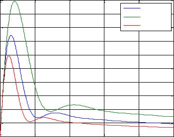
Figure 24. Simulated step responses of the temperature T(0,t) at x = 0 (a) and T(5mm,t) at x = 5mm (b) for a step input of 1°C for aluminum, copper and iron, in the case of a position sensor xcapt = 0 mm.
Complimentary Contributor Copy