The stability is guaranteed if the derivative of the Lyapunov function is negative definite, also known as the reaching condition. Taking the first time derivative from (18) one gets:

uncertainties [33], then Vk will be negative which implies asymptotic stability of the system and Sk (t) and Sk (t) tend to zero as t .

4. Adaptation Law Synthesis

In this section an adaptive scheme based on Lyapunov function for switching feedback control gains is derived. The adaptation law guarantees the system stability regardless of model uncertainty bound. Take the following Lyapunov function

(21) with respect to time and with the sense of (20), one has:

Complimentary Contributor Copy

so the adaptation law can be derived directly from (23) as follow

The switching controller parameters ks and kks in switching control (13) are evaluated

through the adaptive algorithm derived in (24).

As the bound of uncertainty is not available, choosing switching controller gains manually can make chattering effect worst. Therefore, by virtue of adaptation law (24) switching controller parameters assume their gains by making a compromise between chattering suppression and reaching condition.

5. Numerical Studies

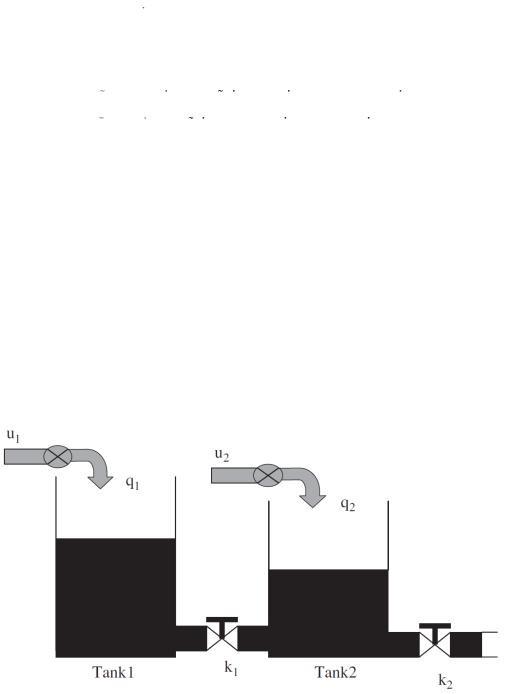
The twin-tanks system comprised of two small tanks mounted above a reservoir which provides storage for the water, Figure 2. Water is pumped into the bottom of each tank by two independent pumps. The pump only increases the liquid level and is not responsible for pumping the water out of the tank [8].

Figure 2. The plant of a liquid-level control system.

The twin-connected tanks system is a nonlinear dynamical system and the governing dynamical equations can be written as [8, 34]

Complimentary Contributor Copy

where h1 and h2 are the total water heads in Tank 1 and Tank 2 respectively, which are the two outputs of interest, and q1 , q2 are the two inflows into the tanks. It is assumed that A1 and A2 are the capacities of Tank-1 and Tank-2 respectively. Both tanks assumed to have the same cross sectional area i.e. A1 A2 A .

It has been seen in [35] that in chemical plants, selecting the flow rate as an input is more effective than using flow as the input. Thus, if the flow rates are considered as the inputs, i.e., q1 u1 and q2 u2 , the system dynamics can be written as

It seems from (25) and (26) that there is a discontinuity at h1 h2 , so desired water level is selected as hd1 hd 2 .

A mathematical model of Twin Tank can be expressed as follows:

because the pumps can only pump water into the tanks. Therefore constraints on the inflow

Complimentary Contributor Copy

A 84 cm2 , k1 16.8 and k2 12 ) shows good stabilization of the water levels in both tanks

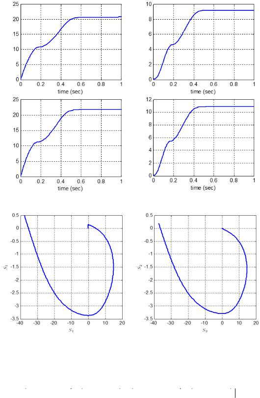
Figs. 3, dashed-line and solid-line represents system’s response and desired trajectory, respectively. The value of inflow in both tanks settles to the steady state values shown in Figure 3, the pumps only increases the liquid level, so their value is always positive.

Figure 3. 2-SMC with PIDDα surface and +20% variation in parameters of Twin Tank system.

Complimentary Contributor Copy

Figure 4. Adaptive parameters versus time.

Figure 5. Phase plot.

Adaptive parameters 1s , k 1s , 2s , k 2s in (24) are estimated as follow with zero initial conditions shown in Figure 4.

Complimentary Contributor Copy