to select the proper 2-D look-up tables, which are used to compute K and T based on the equilibrium actual rail pressure x¯2 and injection timings u¯2. The choice of equilibrium conditions, and thus of the scheduling strategy, is based on a sensitivity analysis of the linear model coefficients. Clearly, the larger the number of operating conditions for the scheduling strategy, the larger the amount of memory to store controller parameters. However, the computational effort does not increase. Namely, the complete set of controller parameters is computed off-line and stored in static look-up tables as a function of the chosen operating conditions.

3.The Control Strategy: Switching of Fractional Order Controllers by Gain Scheduling

To take into account different equilibrium points of the controlled system and to achieve a good trade-off between performance and robustness, a possible solution is to implement switching among fractional order controllers by a scheduling strategy. This is a natural extension of the common approach in automotive applications that frequently employ scheduling of different integer order PI controllers [14, 45, 62]. However, a PI controller is employed for all operating conditions and its tuning is obtained by conventional rules like Ziegler-Nichols [2, 15, 23, 66]. In what follows, the controller parameters depend on the CNG engine working conditions. In other words, for each of these equilibrium points, there is a different fractional order controller that is properly designed to achieve performance and robustness specifications (see Section 4).

Scheduling works as follows. Firstly, the working point is established by the rail pressure and by the average duration, say I, of the injection process, for each value of the approximately constant tank pressure. More specifically, I depends on the injector opening time intervals and on the engine speed. Secondly, the values of the rail pressure and I are considered for the new working point that is required to be reached, and the variation between the two working points is computed. Thirdly, the controller is designed with reference to the set (K, T , τ ) of parameters associated with the new equilibrium point.

This method is used when the variations between the two operating points are bounded by 2 bar for the rail pressure and by 6 seconds for I. However, if the variations are higher than these limit values, then several intermediate rail pressure and I reference values are considered. Then, several sets (K, T , τ ) are determined and several associated controllers are designed. In this way, maps of controller gains are built for the different equilibrium points.

As regards stability of gain scheduling, the pressure reference and I are the scheduling variables subject to step changes between the equilibrium points. Then, the amplitudes of these steps must be limited, because each local linear fractional order controller guarantees stability only close to the equilibrium point. If this holds true, then the initial equilibrium point is in the region of attraction of the changed equilibrium point, and a smooth transition is achieved [20].

If variations of variables are fast, then assessing stability in switching for classical gain scheduling is impossible. In this case, only simulation can be used [59], for which the reader can refer to Section 5. There are recent design approaches, such as those based on linear

Complimentary Contributor Copy

46 Paolo Lino and Guido Maione

parameter-varying systems (LPV) [44], that explicitly take into account time dependency of scheduling variables, so that global closed-loop stability is a priori achieved [45]. However, the number and variation rate of scheduling parameters, as well as complexity of the non-linear model, make the LPV framework inappropriate for the considered application. Namely, analysis and design are complex and the computational effort is high [45].

To better analyze closed-loop stability with respect to variations in working conditions of the injection process, one may refer to the classical D-decomposition methodology [46] that is well known for designing integer order controllers [1] but that was also recently applied to FOPID controllers operating on fractional order systems with delays [16, 18, 29]. Namely, this approach determines all the stabilizing controllers, i.e., the set of controller parameters that guarantee a stable closed-loop system. A stability domain, say D, is defined in the so-called parameter space and the designed controller is associated with a point inside this space. If the point is far from the boundaries of the stability domain, then closed-loop stability is obtained for (small) bounded variations of the controller gains.

To extend the D-decomposition methodology to the case of fractional order controllers, consider the procedure shown by [16, 29]. The starting point is the characteristic equation of a closed loop containing a FOPI controller. If the open-loop transfer function is

where ν is the fractional order of integration, TI = KP /KI , and KP and KI are the proportional and integral gain, respectively. To analyze closed-loop stability, consider the solutions of the fractional order characteristic pseudo-polynomial equation

Then, if all solutions lie in the open left-half of the s-plane (LHP roots), then the closed-loop system is BIBO stable [8, 16, 18].

So, if (KP , KI , ν) D (the set of all stabilizing controllers in the parameter space), then all closed-loop roots are LHP. The domain D is defined by boundaries: the real root boundary (RRB), the infinite root boundary (IRB), and the complex root boundary (CRB)

Complimentary Contributor Copy

which can be used to plot a curve in the 2-D-space (KP , KI ), when ν is fixed and ω is varied from 0 to ∞, since the gains are functions of ω. If a different pair of controller gains is chosen, analogous curves can be drawn in the 2-D-spaces (KP , TI) or (TI , KI ).

The IRB for s → ∞ does not exist, because the condition αn ≤ βn provided in [16] is not satisfied, where αn and βn are, respectively, the integer (in general fractional) orders of the denominator and numerator polynomials of Gp(s) in (11).

To simplify the identification of the complete stability domain D, two steps can be followed. Firstly, one of the parameters (e.g., the order ν) is fixed so that the RRB and CRB boundaries are determined inside the plane defined by the remaining two parameters (e.g., the (KP , KI )-plane). Secondly, the fixed parameter is varied and the complete 3-D stability domain is obtained by sweeping over all the admissible values of the parameter fixed initially.

If the analysis focuses on the plane (KP , KI ), then the boundaries divide it into unstable and stable regions that can be checked by a test point. If a region is stable, then it does not contain any closed-loop root in the closed right-half of the s-plane (RHP root); if a region is unstable, then it includes some RHP root. For the stability check, algorithms were proposed by [18] and [41].

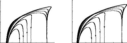
For example, Figure 2a shows the stability regions obtained for ν = 1.3, 1.4, 1.5, 1.6, when a FOPI controller is designed according to the procedure of Section 4, with reference to an equilibrium point defined by K = 165 bar and T = 1.74 s. In particular, the equilibrium points are determined by (K, T )-values corresponding to values of the rail pressure p2 and injection timing tinj , for an engine speed of 2500 rpm. Note that the τ parameter is approximately constant in the whole operating range, if an accurate model of the CNG injection system is considered. Moreover, for a different equilibrium point, a different FOPI controller and a different stability region are defined. Figure 2b shows the case of K = 127 bar and T = 1.97 s. The values of the gains in Figures are indicated but for a multiplying factor of 10−2.

Finally, it is remarked that, for each value of ν, the design point P (marked with × in the Figure 2) lies in the stability region and belongs to a peculiar curve; this curve is called a “relative stability curve” and is obtained by the technique of the phase margin tester [16, 29]. This curve is associated with the specified phase margin P Ms and, for each point, provides a possible gain crossover frequency. Then, the point × determined by the designed values of KP and KI corresponds to the specified gain crossover frequency, ωc. Moving the design point along the relative stability curve changes the controller gains, by keeping the same P Ms while changing ωc. Moreover, another curve (not shown) can be defined for a specified gain margin GMs and passes through a design point that is associated with the phase crossover frequency.

4.Fractional Order Control Design

In this section, the focus is on the P Iν type of controllers, because they recently obtained promising results in mechatronics and automotive control systems. Namely, a systematic design methodology has been applied [24, 26] and is extendable to a wide class of systems. Moreover, this kind of controller is the closest one to PI controllers that are typically employed in industrial contexts [4]. Hence it is quite natural to compare the PI

Complimentary Contributor Copy

Figure 2. Design of FOPI controllers (uc = 5.7, P Ms = 60◦) for two working points and position of design points P in stability regions with respect to stability boundaries (CRB curves) and relative stability curves: (a) K = 165 bar, T = 1.74 s, (b) K = 127 bar,

T = 1.97 s.

to the flexible and robust P Iν , with its high performance due to the additional freedom of choosing the non-integer order ν of integration. The limited complexity of P Iν could also help practitioners to make comparisons with various tuning rules of PI controllers and, above all, to promote their acceptance of the fractional order control paradigm. Finally, as shown below, the choice of the free controller parameters is determined by closed-form formulas that combine a low computational complexity with analytic satisfaction of design specifications (robustness and performance).

The design is guided by basically two ideas:

•the optimality of the closed-loop system, to obtain a system which is a good approximation of an optimal system in a frequency band of interest [19];

•the loop-shaping of the open-loop frequency response, to obtain high robustness to parametric variations and uncertainties, in a sufficiently wide frequency range.

The design obviously requires a realization phase. Namely, implementation of FOC requires approximating the irrational operators that are basic units in Laplace representation of FOC. Then, a rational transfer function must be obtained by a proper approximation technique. Among the available techniques, a continued fractions approach is chosen that shows several benefits:

a)good convergence properties and reduced approximation errors;

b)stability and minimum-phase characteristics, which are very important for control applications;

c)interlacing between real poles and real zeros of the rational transfer function.

Complimentary Contributor Copy

These properties are verified both in the analog and in the discrete domain. The implementation of the approximating transfer functions can be achieved by using interface equipment allowing use of the Matlab/Simulink environment or micro-controllers or low cost components.

4.1.Design Procedure

The design of robust FOPI controllers for each operating point is based on a loopshaping approach. By applying relatively easy closed-form formulas, the methodology directly relates performance and robustness specifications to the values of the controller parameters. More specifically, to achieve robustness to gain variations in a sufficiently wide frequency range around the crossover [26], an integrator of non-integer order ν is particularly suitable. Namely, it leads to a nearly flat phase diagram and a constant slope of the magnitude diagram of the open-loop gain in that range. Moreover, to pursue optimality of the feedback system [19], the open-loop frequency response is so shaped that the gain is high at low frequencies and rolls off at high frequencies to avoid stability problems [61]. A good input-output tracking is obtained in a specified bandwidth.

The proposed design procedure was conceived for controlling plants with transfer function Gp(s) = [26]. In particular, the background idea was inspired by the symmetrical optimum method that is often used to tune integer order PI controllers for electric drives [39]. Subsequently, the effect of time delay τ has been added [24, 25]. To cover a

Here, the controlled plant of a unitary feedback control system is considered, in which

where K is the static dc-gain, T is the time constant of the dominant dynamics and τ is the dead time of the injection system. Moreover, the system includes a FOPI controller that is characterized by a standard proportional element and an integral action of non-integer order

1 < ν < 2:

with TI = KP and where KP and KI are the proportional and integral gain, respectively.

KI

In this way, the open-loop gain G(s) = Gc(s) Gp(s) is:

The non-integer order is chosen 1 < ν < 2 so that an integer unitary integration s−1 is included to allow compensation of disturbances on the plant. The reason for this choice is that, if the non-integer operator sν with 0 < ν < 1 is approximated by a rational transfer function, then a non-zero dc-gain would be obtained by this realization and a steady-state error would occur. Instead, by using 1 < ν < 2, an integer integrator (with order equal to 1) and a non-integer integrator (with order λ = ν − 1 and 0 < λ < 1) ensue. Therefore,

Complimentary Contributor Copy

increased flexibility is gained due to three design parameters (KP , KI , ν), i.e., to one more degree of freedom with respect to a PI controller. However, reliable and effective rules to design and tune the parameters must also be established.

Putting s = jω, the open-loop frequency response (OLFR for brevity) associated with G(s) = Gc(s) Gp(s) is given by:

timality requirement |F (ju)| ≡ 1 is approximated in a sufficiently large bandwidth uB . In theory, however, an optimal feedback system that provides perfect input-output tracking should be achieved only if this holds true for all frequencies. i.e., |G(ju)| 1, u should be verified. Namely, “a feedback system is optimal if and only if the absolute value of the return difference is at least one at all frequencies” [19], but this condition cannot be satisfied by the return difference |1 +G−1(jω)|. Instead, |G(ju)|is shaped around the crossover uc so that a high gain is obtained at low frequencies, whereas it rolls off at high frequencies to avoid stability problems [61]. The appropriate shaping guarantees robust stability and desired performance despite parameter variations in the controlled injection system. Namely, the non-integer order integrator provides a magnitude plot with a fractional slope of −20 dB/decade and a nearly flat phase diagram in a range around uc so that a nearly constant phase margin is achieved in this range.

To synthesize, start by fixing uB where optimal tracking is desired. In particular, a trade-off is reached. Namely, the higher uB is, the lower the rise time in the response of the closed-loop system. Moreover, the lower is uB , the more the crossover uc is shifted toward a centered position in the flat region of the phase characteristic. For the sake of convenience, uB is chosen higher than the plant bandwidth.

Then the normalized crossover frequency is estimated by a commonly used relation [31]: uc [ u1.B7 , u1.B3 ], e.g., uc = u1.B5 . The estimate may be changed inside the indicated

Complimentary Contributor Copy

range to adjust TI . Then, to achieve a specified phase margin P Ms at uc, TI is properly selected. Namely, the phase margin P M = π + G(juc) is:

where ϕ1(uc) and ϕ2(uc) are the first two arguments on the right side of (27). Then, TI is determined to compensate the delay by putting ϕ1(uc) − ϕ2(uc) − uc Tτ = 0 and obtain a closed-form formula:

which represents a direct and easy design relation between the fractional order ν and the specification provided on P Ms. Note that ν > 1 is always obtained for a plant without an integrator. Obviously, at the end of the design procedure, it is always verified that the FOPI controller ensures a nearly flat Bode plot of G(ju), so that the obtained phase margin is nearly constant in a range around uc.

To complete the design procedure, |G−1(juc)|2 = 1 is helpful to get another closedform formula for determining KI :

The (30) also leads to KP = KI TI .

It is to be noted that the value and sign of TI in (28) depend on the choice of ν (i.e., the specified P Ms), which affects C and S, and on the choice of uc (i.e., the specified uB ). Then, if uB is fixed, ν is restricted to allow TI > 0, i.e., a minimum-phase and stable compensated system. This means that restrictions apply on the achievable phase margin. Vice versa, if P Ms is fixed, the same kind of restriction applies on uc. In other words, restrictions apply on the achievable bandwidth. For example, for P Ms = π/4 with ν = 1.5, Table 1 provides the values of TI for several values of the pairs (r, uc), where r is the delay ratio r = τ /T and uc {uB /1.7, uB/1.5, uB/1.3}, with uB = 2π.

Finally, another point must be noted. Given T from the plant model, uc, and ν, the

corresponding to uc = uB /1.5 = 4.1888, τ = 0.18 seconds and T = 1.6857 seconds (r = 0.1068), which are the parameters of the CNG injection system model for a particular working condition. In all cases, τmax > τ so the controller design is possible.

Complimentary Contributor Copy

52 Paolo Lino and Guido Maione

Table 1. Values of TI (s) corresponding to pairs (r, uc) for P Ms = 54◦, 45◦, 36◦ (with

ν = 1.4, 1.5, 1.6)

Table 2. Values of TI and τmax for a given working condition (T = 1.6857 s, τ = 0.18 s)

4.2.Realization

The final step of the design procedure requires realization of the irrational non-integer order operator sν . To this aim, a rational transfer function approximation is required. Many approximation methods exist, starting with the well-known recursive Oustaloup’s technique [48]. Other approaches are based on truncation of continued fraction expansions (CFEs) and interpolation techniques [12, 67] or signal processing techniques [6]. Here, an efficient method is used that derives approximations from the Lagrange’s CFE [33].

This CFE-based method a priori guarantees minimum-phase zeros and stable poles of the approximating rational transfer function and is based on closed-form formulas expressing coefficients of the numerator and denominator polynomials in the transfer function. Moreover, zeros and poles are interlaced on the negative real half-axis [35], and this property also holds for digital realization [32, 34, 36]. This is very important for controller synthesis, because right-half plane (RHP) zeros and RHP poles in the open-loop transfer function imply inherent limitations to the benefits of feedback [17, 60]. More specifically, RHP poles imply constrained large gain bandwidth, which leads to a highly amplified sensor noise at the input to the plant. Finally, the method can obtain a reduced approximation

Complimentary Contributor Copy