DISK TRANSFER RATES

As with many aspects of computing, published performance numbers for disks are not the same as real-world performance numbers. Stated transfer rates are always lower than effective transfer rates, for example. The transfer rate may be the rate at which bits can be read from the magnetic media by the disk head, but that is different from the rate at which blocks are delivered to the operating system.

Tapes are used mainly for backup, for storage of infrequently used information, and as a medium for transferring information from one system to another.

A tape is kept in a spool and is wound or rewound past a read –write head. Moving to the correct spot on a tape can take minutes, but once positioned, tape drives can write data at speeds comparable to disk drives. Tape capacities vary greatly, depending on the particular kind of tape drive, with current capacities exceeding several terabytes. Some tapes have built-in compression that can more than double the effective storage. Tapes and their drivers are usually categorized by width, including 4, 8, and 19 millimeters and 1/4 and 1/2 inch. Some are named according to technology, such as LTO-5 and SDLT.

10.2 Disk Structure

Modern magnetic disk drives are addressed as large one-dimensional arrays of logical blocks, where the logical block is the smallest unit of transfer. The size of a logical block is usually 512 bytes, although some disks can be low-level formatted to have a different logical block size, such as 1,024 bytes. This option is described in Section 10.5.1. The one-dimensional array of logical blocks is mapped onto the sectors of the disk sequentially. Sector 0 is the first sector of the first track on the outermost cylinder. The mapping proceeds in order through that track, then through the rest of the tracks in that cylinder, and then through the rest of the cylinders from outermost to innermost.

By using this mapping, we can—at least in theory —convert a logical block number into an old-style disk address that consists of a cylinder number, a track number within that cylinder, and a sector number within that track. In practice, it is difficult to perform this translation, for two reasons. First, most disks have some defective sectors, but the mapping hides this by substituting spare sectors from elsewhere on the disk. Second, the number of sectors per track is not a constant on some drives.

Let’s look more closely at the second reason. On media that use constant linear velocity (CLV), the density of bits per track is uniform. The farther a track is from the center of the disk, the greater its length, so the more sectors it can hold. As we move from outer zones to inner zones, the number of sectors per track decreases. Tracks in the outermost zone typically hold 40 percent more sectors than do tracks in the innermost zone. The drive increases its rotation speed as the head moves from the outer to the inner tracks to keep the same rate of data moving under the head. This method is used in CD-ROM

and DVD-ROM drives. Alternatively, the disk rotation speed can stay constant; in this case, the density of bits decreases from inner tracks to outer tracks to keep the data rate constant. This method is used in hard disks and is known as constant angular velocity (CAV).

The number of sectors per track has been increasing as disk technology improves, and the outer zone of a disk usually has several hundred sectors per track. Similarly, the number of cylinders per disk has been increasing; large disks have tens of thousands of cylinders.

10.3 Disk Attachment

Computers access disk storage in two ways. One way is via I/O ports (or host-attached storage); this is common on small systems. The other way is via a remote host in a distributed file system; this is referred to as network-attached storage.

10.3.1Host-Attached Storage

Host-attached storage is storage accessed through local I/O ports. These ports use several technologies. The typical desktop PC uses an I/O bus architecture called IDE or ATA. This architecture supports a maximum of two drives per I/O bus. A newer, similar protocol that has simplified cabling is SATA.

High-end workstations and servers generally use more sophisticated I/O architectures such as fibre channel (FC), a high-speed serial architecture that can operate over optical fiber or over a four-conductor copper cable. It has two variants. One is a large switched fabric having a 24-bit address space. This variant is expected to dominate in the future and is the basis of storage-area networks (SANs), discussed in Section 10.3.3. Because of the large address space and the switched nature of the communication, multiple hosts and storage devices can attach to the fabric, allowing great flexibility in I/O communication. The other FC variant is an arbitrated loop (FC-AL) that can address 126 devices (drives and controllers).

A wide variety of storage devices are suitable for use as host-attached storage. Among these are hard disk drives, RAID arrays, and CD, DVD, and tape drives. The I/O commands that initiate data transfers to a host-attached storage device are reads and writes of logical data blocks directed to specifically identified storage units (such as bus ID or target logical unit).

10.3.2Network-Attached Storage

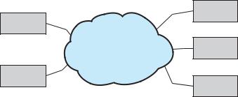
A network-attached storage (NAS) device is a special-purpose storage system that is accessed remotely over a data network (Figure 10.2). Clients access network-attached storage via a remote-procedure-call interface such as NFS for UNIX systems or CIFS for Windows machines. The remote procedure calls (RPCs) are carried via TCP or UDP over an IP network —usually the same localarea network (LAN) that carries all data traffic to the clients. Thus, it may be easiest to think of NAS as simply another storage-access protocol. The networkattached storage unit is usually implemented as a RAID array with software that implements the RPC interface.

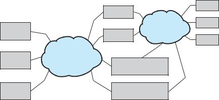
Figure 10.3 Storage-area network.

access time and large disk bandwidth. For magnetic disks, the access time has two major components, as mentioned in Section 10.1.1. The seek time is the time for the disk arm to move the heads to the cylinder containing the desired sector. The rotational latency is the additional time for the disk to rotate the desired sector to the disk head. The disk bandwidth is the total number of bytes transferred, divided by the total time between the first request for service and the completion of the last transfer. We can improve both the access time and the bandwidth by managing the order in which disk I/O requests are serviced.

Whenever a process needs I/O to or from the disk, it issues a system call to the operating system. The request specifies several pieces of information:

•Whether this operation is input or output

•What the disk address for the transfer is

•What the memory address for the transfer is

•What the number of sectors to be transferred is

If the desired disk drive and controller are available, the request can be serviced immediately. If the drive or controller is busy, any new requests for service will be placed in the queue of pending requests for that drive. For a multiprogramming system with many processes, the disk queue may often have several pending requests. Thus, when one request is completed, the operating system chooses which pending request to service next. How does the operating system make this choice? Any one of several disk-scheduling algorithms can be used, and we discuss them next.

10.4.1FCFS Scheduling

The simplest form of disk scheduling is, of course, the first-come, first-served (FCFS) algorithm. This algorithm is intrinsically fair, but it generally does not provide the fastest service. Consider, for example, a disk queue with requests for I/O to blocks on cylinders

98, 183, 37, 122, 14, 124, 65, 67,

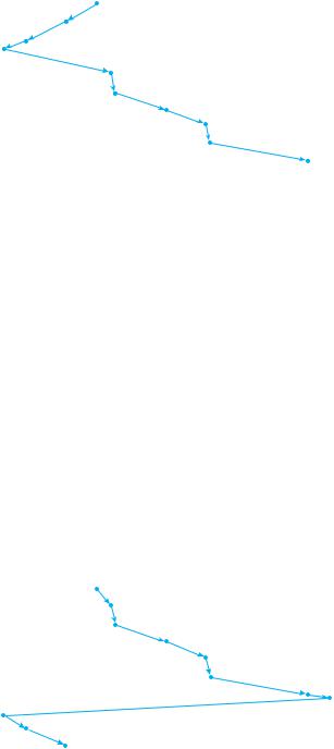
Figure 10.4 FCFS disk scheduling.

in that order. If the disk head is initially at cylinder 53, it will first move from 53 to 98, then to 183, 37, 122, 14, 124, 65, and finally to 67, for a total head movement of 640 cylinders. This schedule is diagrammed in Figure 10.4.

The wild swing from 122 to 14 and then back to 124 illustrates the problem with this schedule. If the requests for cylinders 37 and 14 could be serviced together, before or after the requests for 122 and 124, the total head movement could be decreased substantially, and performance could be thereby improved.

10.4.2 SSTF Scheduling

It seems reasonable to service all the requests close to the current head position before moving the head far away to service other requests. This assumption is the basis for the shortest-seek-time-first (SSTF) algorithm. The SSTF algorithm selects the request with the least seek time from the current head position. In other words, SSTF chooses the pending request closest to the current head position.

For our example request queue, the closest request to the initial head position (53) is at cylinder 65. Once we are at cylinder 65, the next closest request is at cylinder 67. From there, the request at cylinder 37 is closer than the one at 98, so 37 is served next. Continuing, we service the request at cylinder 14, then 98, 122, 124, and finally 183 (Figure 10.5). This scheduling method results in a total head movement of only 236 cylinders —little more than one-third of the distance needed for FCFS scheduling of this request queue. Clearly, this algorithm gives a substantial improvement in performance.

SSTF scheduling is essentially a form of shortest-job-first (SJF) scheduling; and like SJF scheduling, it may cause starvation of some requests. Remember that requests may arrive at any time. Suppose that we have two requests in the queue, for cylinders 14 and 186, and while the request from 14 is being serviced, a new request near 14 arrives. This new request will be serviced next, making the request at 186 wait. While this request is being serviced, another request close to 14 could arrive. In theory, a continual stream of requests near one another could cause the request for cylinder 186 to wait indefinitely.

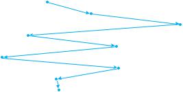
Figure 10.5 SSTF disk scheduling.

This scenario becomes increasingly likely as the pending-request queue grows longer.

Although the SSTF algorithm is a substantial improvement over the FCFS algorithm, it is not optimal. In the example, we can do better by moving the head from 53 to 37, even though the latter is not closest, and then to 14, before turning around to service 65, 67, 98, 122, 124, and 183. This strategy reduces the total head movement to 208 cylinders.

10.4.3SCAN Scheduling

In the SCAN algorithm, the disk arm starts at one end of the disk and moves toward the other end, servicing requests as it reaches each cylinder, until it gets to the other end of the disk. At the other end, the direction of head movement is reversed, and servicing continues. The head continuously scans back and forth across the disk. The SCAN algorithm is sometimes called the elevator algorithm, since the disk arm behaves just like an elevator in a building, first servicing all the requests going up and then reversing to service requests the other way.

Let’s return to our example to illustrate. Before applying SCAN to schedule the requests on cylinders 98, 183, 37, 122, 14, 124, 65, and 67, we need to know the direction of head movement in addition to the head’s current position. Assuming that the disk arm is moving toward 0 and that the initial head position is again 53, the head will next service 37 and then 14. At cylinder 0, the arm will reverse and will move toward the other end of the disk, servicing the requests at 65, 67, 98, 122, 124, and 183 (Figure 10.6). If a request arrives in the queue just in front of the head, it will be serviced almost immediately; a request arriving just behind the head will have to wait until the arm moves to the end of the disk, reverses direction, and comes back.

Assuming a uniform distribution of requests for cylinders, consider the density of requests when the head reaches one end and reverses direction. At this point, relatively few requests are immediately in front of the head, since these cylinders have recently been serviced. The heaviest density of requests