Now that you understand the fundamental concepts of operating systems (CPU scheduling, memory management, processes, and so on), we are in a position to examine how these concepts have been applied in several older and highly influential operating systems. Some of them (such as the XDS-940 and the THE system) were one-of-a-kind systems; others (such as OS/360) are widely used. The order of presentation highlights the similarities and differences of the systems; it is not strictly chronological or ordered by importance. The serious student of operating systems should be familiar with all these systems.

In the bibliographical notes at the end of the chapter, we include references to further reading about these early systems. The papers, written by the designers of the systems, are important both for their technical content and for their style and flavor.

CHAPTER OBJECTIVES

•To explain how operating-system features migrate over time from large computer systems to smaller ones.

•To discuss the features of several historically important operating systems.

20.1Feature Migration

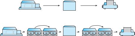
One reason to study early architectures and operating systems is that a feature that once ran only on huge systems may eventually make its way into very small systems. Indeed, an examination of operating systems for mainframes and microcomputers shows that many features once available only on mainframes have been adopted for microcomputers. The same operating-system concepts are thus appropriate for various classes of computers: mainframes, minicomputers, microcomputers, and handhelds. To understand modern operating systems, then, you need to recognize the theme of feature migration and the long history of many operating-system features, as shown in Figure 20.1.

A good example of feature migration started with the Multiplexed Information and Computing Services (MULTICS) operating system. MULTICS was

887

Figure 20.1 Migration of operating-system concepts and features.

developed from 1965 to 1970 at the Massachusetts Institute of Technology (MIT) as a computing utility. It ran on a large, complex mainframe computer (the GE 645). Many of the ideas that were developed for MULTICS were subsequently used at Bell Laboratories (one of the original partners in the development of MULTICS) in the design of UNIX. The UNIX operating system was designed around 1970 for a PDP-11 minicomputer. Around 1980, the features of UNIX became the basis for UNIX-like operating systems on microcomputers; and these features are included in several more recent operating systems for microcomputers, such as Microsoft Windows, Windows XP, and the Mac OS X operating system. Linux includes some of these same features, and they can now be found on PDAs.

20.2 Early Systems

We turn our attention now to a historical overview of early computer systems. We should note that the history of computing starts far before “computers” with looms and calculators. We begin our discussion, however, with the computers of the twentieth century.

Before the 1940s, computing devices were designed and implemented to perform specific, fixed tasks. Modifying one of those tasks required a great deal of effort and manual labor. All that changed in the 1940s when Alan Turing and John von Neumann (and colleagues), both separately and together, worked on the idea of a more general-purpose stored program computer. Such a machine

has both a program store and a data store, where the program store provides instructions about what to do to the data.

This fundamental computer concept quickly generated a number of general-purpose computers, but much of the history of these machines is blurred by time and the secrecy of their development during World War II. It is likely that the first working stored-program general-purpose computer was the Manchester Mark 1, which ran successfully in 1949. The first commercial computer — the Ferranti Mark 1, which went on sale in 1951—was it offspring.

Early computers were physically enormous machines run from consoles. The programmer, who was also the operator of the computer system, would write a program and then would operate the program directly from the operator’s console. First, the program would be loaded manually into memory from the front panel switches (one instruction at a time), from paper tape, or from punched cards. Then the appropriate buttons would be pushed to set the starting address and to start the execution of the program. As the program ran, the programmer/operator could monitor its execution by the display lights on the console. If errors were discovered, the programmer could halt the program, examine the contents of memory and registers, and debug the program directly from the console. Output was printed or was punched onto paper tape or cards for later printing.

20.2.1Dedicated Computer Systems

As time went on, additional software and hardware were developed. Card readers, line printers, and magnetic tape became commonplace. Assemblers, loaders, and linkers were designed to ease the programming task. Libraries of common functions were created. Common functions could then be copied into a new program without having to be written again, providing software reusability.

The routines that performed I/O were especially important. Each new I/O device had its own characteristics, requiring careful programming. A special subroutine —called a device driver —was written for each I/O device. A device driver knows how the buffers, flags, registers, control bits, and status bits for a particular device should be used. Each type of device has its own driver. A simple task, such as reading a character from a paper-tape reader, might involve complex sequences of device-specific operations. Rather than writing the necessary code every time, the device driver was simply used from the library.

Later, compilers for FORTRAN, COBOL, and other languages appeared, making the programming task much easier but the operation of the computer more complex. To prepare a FORTRAN program for execution, for example, the programmer would first need to load the FORTRAN compiler into the computer. The compiler was normally kept on magnetic tape, so the proper tape would need to be mounted on a tape drive. The program would be read through the card reader and written onto another tape. The FORTRAN compiler produced assembly-language output, which then had to be assembled. This procedure required mounting another tape with the assembler. The output of the assembler would need to be linked to supporting library routines. Finally, the binary object form of the program would be ready to execute. It could be loaded into memory and debugged from the console, as before.

890 Chapter 20 Influential Operating Systems

A significant amount of setup time could be involved in the running of a job. Each job consisted of many separate steps:

1. Loading the FORTRAN compiler tape

2. Running the compiler

3. Unloading the compiler tape

4. Loading the assembler tape

5. Running the assembler

6. Unloading the assembler tape

7. Loading the object program

8. Running the object program

If an error occurred during any step, the programmer/operator might have to start over at the beginning. Each job step might involve the loading and unloading of magnetic tapes, paper tapes, and punch cards.

The job setup time was a real problem. While tapes were being mounted or the programmer was operating the console, the CPU sat idle. Remember that, in the early days, few computers were available, and they were expensive. A computer might have cost millions of dollars, not including the operational costs of power, cooling, programmers, and so on. Thus, computer time was extremely valuable, and owners wanted their computers to be used as much as possible. They needed high utilization to get as much as they could from their investments.

20.2.2 Shared Computer Systems

The solution was twofold. First, a professional computer operator was hired. The programmer no longer operated the machine. As soon as one job was finished, the operator could start the next. Since the operator had more experience with mounting tapes than a programmer, setup time was reduced. The programmer provided whatever cards or tapes were needed, as well as a short description of how the job was to be run. Of course, the operator could not debug an incorrect program at the console, since the operator would not understand the program. Therefore, in the case of program error, a dump of memory and registers was taken, and the programmer had to debug from the dump. Dumping the memory and registers allowed the operator to continue immediately with the next job but left the programmer with the more difficult debugging problem.

Second, jobs with similar needs were batched together and run through the computer as a group to reduce setup time. For instance, suppose the operator received one FORTRAN job, one COBOL job, and another FORTRAN job. If she ran them in that order, she would have to set up for FORTRAN (load the compiler tapes and so on), then set up for COBOL, and then set up for FORTRAN again. If she ran the two FORTRAN programs as a batch, however, she could setup only once for FORTRAN, saving operator time.

loader

control card interpreter

user program area

Figure 20.2 Memory layout for a resident monitor.

But there were still problems. For example, when a job stopped, the operator would have to notice that it had stopped (by observing the console), determine why it stopped (normal or abnormal termination), dump memory and register (if necessary), load the appropriate device with the next job, and restart the computer. During this transition from one job to the next, the CPU sat idle.

To overcome this idle time, people developed automatic job sequencing. With this technique, the first rudimentary operating systems were created. A small program, called a resident monitor, was created to transfer control automatically from one job to the next (Figure 20.2). The resident monitor is always in memory (or resident).

When the computer was turned on, the resident monitor was invoked, and it would transfer control to a program. When the program terminated, it would return control to the resident monitor, which would then go on to the next program. Thus, the resident monitor would automatically sequence from one program to another and from one job to another.

But how would the resident monitor know which program to execute? Previously, the operator had been given a short description of what programs were to be run on what data. Control cards were introduced to provide this information directly to the monitor. The idea is simple. In addition to the program or data for a job, the programmer supplied control cards, which contained directives to the resident monitor indicating what program to run. For example, a normal user program might require one of three programs to run: the FORTRAN compiler (FTN), the assembler (ASM), or the user’s program (RUN). We could use a separate control card for each of these:

$FTN —Execute the FORTRAN compiler. $ASM —Execute the assembler.

$RUN —Execute the user program.

These cards tell the resident monitor which program to run.