Patterson, Bailey - Solid State Physics Introduction to theory

For high temperatures (and/or weak magnetic fields, so only the first two terms of the expansion of the exponential need be retained) we can write

2 where peff = g[S(S+1)]1/2 is called the effective magneton number. Equation (7.12) is the Curie law. It expresses the (1/T) dependence of the magnetic susceptibility at high temperature. Note that when H → 0, (7.12) is an exact consequence of (7.11).

It is convenient to have an expression for the magnetization of paramagnets that is valid at all temperatures and magnetic fields.

If we define

With a little elementary manipulation, it is possible to perform the sums indicated in (7.14):

or

2A temperature-independent contribution known as van Vleck paramagnetism may also be important for some materials at low temperature. It may occur due to the effect of excited states that can be treated by second-order perturbation theory. It is commonly important when first-order terms vanish. See Ashcroft and Mermin [7.2 p. 653].

(i.e. because of exchange coupling between the spins as we will discuss in Sect. 7.2). They also have more complex domain effects that will not be discussed.

Examples of elements that show spontaneous magnetism or ferromagnetism are

(1) transition or iron group elements (e.g. Fe, Ni, Co), (2) rare earth group elements (e.g. Gd or Dy), and (3) many compounds and alloys. Further examples are given in Sect. 7.3.2.

The Weiss theory is a mean field theory and is perhaps the simplest way of discussing the appearance of the ferromagnetic state. First, what is mean field theory? Basically, mean field theory is a linearized theory in which the Hamiltonian products of operators representing dynamical observables are approximated by replacing these products by a dynamical observable times the mean or average value of a dynamic observable. The average value is then calculated self-consistently from this approximated Hamiltonian. The nature of this approximation is such that thermodynamic fluctuations are ignored. Mean field theory is often used to get an idea as to what structures or phases are present as the temperature and other parameters are varied. It is almost universally used as a first approximation, although, as discussed below, it can even be qualitatively wrong (in, for example, predicting a phase transition where there is none).

The Weiss mean field theory does the main thing that we want a theory of the magnetic state to do. It predicts a phase transition. Unfortunately, the quantitative details of real phase transitions are typically not what the Weiss theory says they should be. Still, it has several advantages:

1.It provides a comprehensive if at times only qualitative description of most magnetic materials. The Weiss theory (augmented with the concept of domains) is still the most important theory for a practical discussion of many types of magnetic behavior. Many experimental results are still presented within the context of this theory, and so in order to read the experimental papers it is necessary to understand Weiss theory.

2.It is rigorous for infinite-range interactions between spins (which never occur in practice).

3.The Weiss theory originally postulated a mysterious molecular field that was the “real” cause of the ordered magnetic state. This molecular field was later given an explanation based on the exchange effects described by the Heisenberg Hamiltonian (see Sect. 7.2). The Weiss theory gives a very simple way of relating the occurrence of a phase transition to the description of a magnetic system by the Heisenberg Hamiltonian. Of course, the way it relates these two is only qualitatively correct. However, it is a good starting place for more general theories that come closer to describing the behavior of the actual magnetic systems.3

3Perhaps the best simple discussion of the Weiss and related theories is contained in the book by J. S. Smart [92], which can be consulted for further details. By using two sublattices, it is possible to give a similar (to that below) description of antiferromagnetism. See Sect. 7.1.3.

If these equations are identical, then they must have the same slope as a′ → 0. That is, we require

Using the known behavior of BS(a′) as a′ → 0, we find that condition (7.23) gives

Equation (7.24) provides the relationship between the Curie constant Tc and the Weiss molecular field constant γ. Note that, as expected, if γ = 0, then Tc = 0 (i.e. if γ → 0, there is no phase transition). Further, numerical evaluation shows that if T > Tc, (7.21) and (7.22) with H = 0 have a common solution for M only if M = 0. However, for T < Tc, numerical evaluation shows that they have a common solution M ≠ 0, corresponding to the spontaneous magnetization that occurs when the molecular field overwhelms thermal effects.

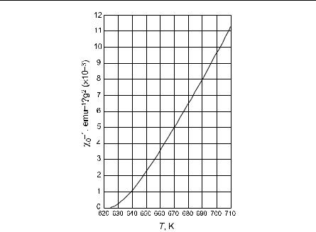
There is another Curie temperature besides Tc. This is the so-called paramagnetic Curie temperature θ that enters into the equation for the high-temperature behavior of the magnetic susceptibility. Within the context of the Weiss theory, these two temperatures turn out to be the same. However, if one makes an experimental determination of Tc (from the transition temperature) and of θ from the high-temperature magnetic susceptibility, θ and Tc do not necessarily turn out to be identical (See Fig. 7.1). We obtain an explicit expression for θ below.

For μ0HSgμB/kT << 1 we have (by (7.17) and (7.18))

For ferromagnetic materials we need to make the replacement H → H + γM so that M = C′H + C′γM or

Substituting the definition of C′, we find that (7.26) gives for the susceptibility

where

C 0 B

≡ the Curie–Weiss = μ Ng2μ2 S(S +1) ,

3k

θ ≡ the paramagnetic Curie temperature = μ0 Ng 2S(S +1) μ2γ . 3k B

which should not be confused with the magnetic moment. It is also convenient to define a quantity Jex by

where Z is the number of nearest neighbors in the lattice of interest, and Jex is the exchange integral. Compare this to (7.95), which is the same. That is, we will see that (7.31) makes sense from the discussion of the physical origin of the molecular field.

Finally, let us define

and

τ = T / Tc .

With these definitions, a little manipulation shows that (7.29) is

Equations (7.30) and (7.33) can be solved simultaneously for m (which is proportional to the magnetization). With b0 equal to zero (i.e. H = 0) we combine (7.30) and (7.33) to give a single equation that determines the spontaneous magnetization:

A plot similar to that yielded by (7.34) is shown in Fig. 7.16 (H = 0). The fit to experiment of the molecular field model is at least qualitative. Some classic results for Ni by Weiss and Forrer as quoted by Kittel [7.39 p. 448] yield a reasonably good fit.

We have reached the point where we can look at sufficiently fine details to see how the molecular field theory gives predictions that do not agree with experiment. We can see this by looking at the solutions of (7.34) as τ → 0 (i.e. T << Tc) and as τ → 1 (i.e. T → Tc).

We know that for any y that BS(y) is given by (7.16). We also know that

Since for large X

coth X 1+ 2e−2X ,

Perhaps the most dramatic failure of the Weiss molecular field theory occurs when we consider the specific heat. As we will see, the Weiss theory flatly predicts that the specific heat (with no external field) should vanish for temperatures above the Curie temperature. Experiment, however, says nothing of the sort. There is a small residual specific heat above the Curie temperature. This specific heat drops off with temperature. The reason for this failure of the Weiss theory is the neglect of short-range ordering above the Curie temperature.

Let us now look at the behavior of the Weiss predictions for the magnetic specific heat in a little more detail. The energy of a spin in a γM field in the z direction due to the molecular field is

Thus the internal energy U obtained by averaging Ei for N spins is,

where the factor 1/2 comes from the fact that we do not want to count bonds twice, and M = −NgμB Siz / has been used.

The specific heat in zero magnetic field is then given by

For T > Tc, M = 0 (with no external magnetic field) and so the specific heat vanishes, which contradicts experiment.

The precise behavior of the magnetic specific heat just above the Curie temperature is of more than passing interest. Experimental results suggest that the specific heat should exhibit a logarithmic singularity or near logarithmic singularity as T → Tc. The Weiss theory is inadequate even to begin attacking this problem.

Antiferromagnetism, Ferrimagnetism, and Other Types

of Magnetic Order (B)

Antiferromagnetism is similar to ferromagnetism except that the lowest-energy state involves adjacent spins that are antiparallel rather than parallel (but see the end of this section). As we will see, the reason for this is a change in sign (compared to ferromagnetism) for the coupling parameter or exchange integral.

Ferrimagnetism is similar to antiferromagnetism except that the paired spins do not cancel and thus the lowest-energy state has a net spin.

Examples of antiferromagnetic substances are FeO and MnO. Further examples are given in Sect. 7.3.2. The temperature at which an antiferromagnetic substance becomes paramagnetic is known as the Néel temperature.

Examples of ferrimagnetism are MnFe2O4 and NiFe2O7. Further examples are also given in Sect. 7.3.2.