Добавил:

Upload Опубликованный материал нарушает ваши авторские права? Сообщите нам.

Вуз:

Национальный авиационный университет

Предмет:

[НЕСОРТИРОВАННОЕ]

Файл:

Higher_Mathematics_Part_3

.pdf

Скачиваний:

306

Добавлен:

19.02.2016

Размер:

9.11 Mб

Скачать

☆

<<< < Предыдущая 1 2 3 4 5 6 7 8 9 10 11 12 13 14 15 16 17 1819 / 2419 20 21 22 23 24 > Следующая >>>

	(2;1)
7.4.20.	∫	(3x2 y2 + y3 + 4x)dx + (2x3 y + 3xy2 )dy.
	(0; 0)
	(3;3)
7.4.21.	∫	(4x3 y2 + 2xy3 )dx + (2 yx4 + 3x2 y2 + 4 y3 )dy.
	(−2; 0)
	(4; 5)
7.4.22.	∫	(4x3 y2 + y2 )dx + (2x4 y + 2xy + 10 y −1)dy.
	(2; 0)
	(2; 0; 2)
7.4.23.	∫	( y + 2z + 4)dx + (x + 3z − 2)dy + (2x + 3y + 1)dz .
	(0;1; 1)
	(3;1)
7.4.24.	∫	( y2 + 6y)dx + (2xy + 6x − 10y)dy .
	(1; 0)
	(1; 2)
7.4.25.	∫	(2xy2 + y + 4)dx + (2x2 y + x)dy .
	(−1; 0)
	(4; 4)
7.4.26.	∫	(x−1 + 2xy2 )dx + ( y−1 + 2x2 y)dy = 0 .
	(1; 2)
	(1; 4)
7.4.27.	∫	(3y2 + 5y)dx + (6xy + 5x − 2y)dy.
	(0; 2)
	(1; 4; 0)
7.4.28.	∫	( y3 − z2 + 2x)dx + (3xy2 + z)dy + ( y − 2xz)dz.
	(0;1; 2)
	(2;5)
7.4.29.	∫	(4xy −15x2 y)dx + (2x2 − 5x3 + 4)dy.
	(0;1)
	(2;3)
7.4.30.	∫	(4x3 y3 + 3x2 y2 + 2xy)dx + (3x4 y2 + 2x3 y + x2 )dy.
	(0;1)
		Micromodule 8
BASIC THEORETICAL INFORMATION. SURFACE INTEGRALS

Surface integrals of the first and of the second type. Properties and evaluation. Ostrograsky-Gauss formula. Stokes’ formula.

Key words: smooth surface — гладка поверхня, surface integral of the first type — поверхневий інтеграл першого роду, surface integral of the second

181

http://vk.com/studentu_tk, http://studentu.tk/

type — поверхневий інтеграл другого роду, bilateral or orientable surface — двостороння або орієнтовна поверхня, unilateral or nonorientable surface —

одностороння або неорієнтовна поверхня, oriented surface — орієнтовна поверхня, upper side of a surface — верхня сторона поверхні, lower side of a surface — нижня сторона поверхні.

Literature: [9, сhapter 10, § 4], [15, сhapter 12, section 12.4], [16, сhapter 15, § 5—8], [17, сhapter 3, § 11—12].

8.1. Surface Integrals of the First Type. Basic Concepts

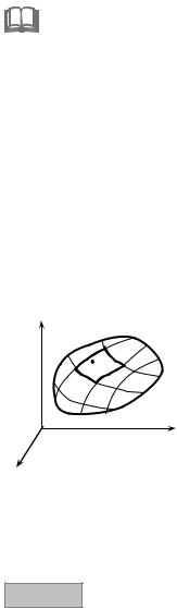
Let the continuous function u = f (x, y, z) on a smooth surface σ be given.

(The surface is called smooth if at each its point a tangent plane changing the position continuously from point to point exists). We’ll divide the surface into n

elementary parts σk ( k = 1, 2, …, n ) via the grid of arbitrary curves, choose in

each part σk any point Mk (xk ,			yk , zk ) , calculate value of the function at this
point and form the integral sum			n
			n
		Sn	= ∑ f (xk ,	yk , zk )Δσk ,			(8.1)
			k =1
where Δσk is the area of k-th element of the surface σk						(Fig. 8.1). We’ll denote
diameter of elementary area of a surface σk as					dk , where λ = max dk is the
greatest of diameters dk .							1≤ k ≤ n
greatest of diameters dk .			If there exists the finite limit of the integral
z			If there exists the finite limit of the integral
z	σ		sum (8.1) while λ → 0			and this limit does not
	σ		sum (8.1) while λ → 0			and this limit does not
	σi		depend on	the	partition of		the surface in
	σi		elementary	parts	σk	and on the choice of
	Mi		elementary	parts	σk	and on the choice of
			points Mk (xk , yk , zk ) on σk ,				then this limit is
			called the Surface integral of the first type of
О			the function	f (x,	y, z)	over the surface and it
О		у	is denoted ∫∫ f (x,		y, z)dσ.
		у	is denoted ∫∫ f (x,		y, z)dσ.
х			σ
х			So, by definition
	Fig. 8.1					n
	Fig. 8.1		∫∫ f (x, y, z)dσ = lim			∑ f (xk , yk , zk )Δσk .
			∫∫ f (x, y, z)dσ = lim			∑ f (xk , yk , zk )Δσk .
			σ		λ→0 k =1

Value of this integral does not depend on the choice of the side of a surface σ on which integration is realized.

Theorem If the continuous function f (x, y, z) on the smooth surface σ is defined, then the surface integral of the first type exists.

182

http://vk.com/studentu_tk, http://studentu.tk/

8.2. Evaluation of the Surface Integral of the First Type

Evaluation of the surface integral of the

evalulation of the double integral.

Let a smooth surface σ be defined by equations z = z(x, y) . We’ll assume that this

surface is biunique projected to the domain D of the plane Оху and that the functions

z(x, y) , z′	(x,	y) ,	z′	(x, y)	are continuous
x		D.	y
in the domain		D.	Then the		correspondence

between an element of a the surface dσ and an element of the area dxdy (Fig. 8.2) exists in the form of formula:

dσ =	dσxy	=	dxdy	,
	cos γ(M (x, y, z))		cos γ(M (x, y, z))

where γ(M ) is an angle between the normal

first type is	reduced	to the
z	G	γ
G	k
n
	M
dσ
O		y
		y

dσxy

n of the surface at the point

M (x, y,

z) and

Fig. 8.2

the the axis Oz.

n = {z′

(x,

y),

z′

(x, y), − 1} ,

In our case it

possible

take

that

then

n k

z′

0 + z

′ 0 − 1 1

cos γ(M (x, y, z))

and

the

′

1+ (zx )

+ (zy )

+ (zx )

+ (zy )

surface integral of the first

type is evaluated by formula

∫∫				∫∫		x	y
	f (x,	y, z)dσ =			f (x, y,	z(x, y)) 1+ (z′ )2 + (z′ )2 dxdy. (8.2)
σ				D
If, for example,		the	smooth		surface	is defined by	equation x = x( y, z) ,
projected in domain		Dyz	of plane Oyz then surface integral of the first type is
calculated by formula

∫∫		∫∫		y	z
	f (x, y, z)dσ =		f (x( y, z), y, z)	1+ (x′ )2	+ (x′ )2 dydz.
σ		Dyz

8.3. Surface Integrals of the Second Type. The Basic Concepts

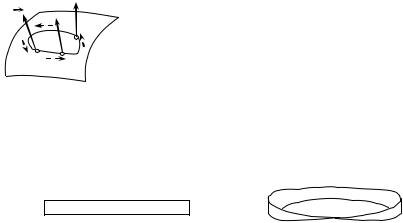
Let’s consider the concept of a bilateral or orientable surface. We’ll take any point M of a smooth surface σ and construct a normal n at this point. Let’s move a point M on any closed oriented contour L together with a vector n , which remains any time normal to a surface σ . If the normal does not change

183

http://vk.com/studentu_tk, http://studentu.tk/

n	the direction after detour round the contour L, the
	surface is called orientable (Fig. 8.3) and if the normal

Lchanges direction to opposite, the surface is called unilateral or nonorientable.

М	Examples of orientable surfaces are the plane,
	sphere, a paraboloid etc. In general, any surface defined
Fig. 8.3	by the equation z = f (x, y) , where f (x, y) , fx′(x, y) ,
Fig. 8.3	f y′ (x, y) are continuous functions in the domain D of

the plane Оху, are orientable. The example of a nonorientable surface is so-called cross-cap (Mobius strip) being the result of pasting sides AB and CD of rectangular АВCD (Fig. 8.4, a) so that the point A is combined with the point C and the point B is combined with the point D (Fig. 8.4, b)

ВС

АD

Fig. 8.4

Let the function R(x, y, z) continuous at the points of the oriented surface

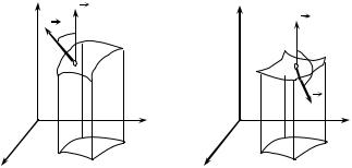
σ be given. We’ll select the certain side of this surface (in this case the surface is called oriented one.). So, if a normal to the selected side forms an acute angle with the axis Оz ( cos γ > 0 ), then the selected side is called upper side of the

surface (Fig. 8.5, a). If a normal to the selected side forms an obtuse angle with the axis Оz ( cos γ < 0 ), then the selected side is called the lower side of the

surface (Fig. 8.5, b). Divide the surface into n elementary parts σk ( k = 1, 2, …, n ) via the grid of arbitrary curves, choose in each part σk any point Mk (xk , yk , zk )

and calculate value of the function at this point. We’ll designate a projection of area σk on the coordinate plane Оху as Dk . Let S(Dk ) be the area of the

projection Dk . We’ll denote Sk = S(Dk ) , if the upper side of a surface is selected, and Sk = −S(Dk ) , if the lower side of a surface is selected . We’ll form the integral sum

n
Sn = ∑ R(xk , yk , zk ) Sk .		(8.3)
k =1
Also we’ll designate a diameter of elementary domain of a surface		σk as
dk , where λ = max dk is the greatest of diameters dk .
1≤k ≤n	λ → 0 and this
If there exists the finite limit of the integral sum 9) while	λ → 0 and this

limit does not depend on the partition of the surface in elementary parts σk , and on the choice of points Mk (xk , yk , zk ) on σk , then this limit is called the

184

http://vk.com/studentu_tk, http://studentu.tk/

surface integral of the second type of the function R(x, y, z) over the surface and it is designated as ∫∫ R(x, y, z)dxdy.

		σ
z		k		z
	n	k		k
	n	σk		k
	γ	σk
		Mk		σk Mk γ
				σk Mk γ
					n
О		у		О	у
		у			у
		+		–
х				х
		a		b
			Fig. 8.5
So, by definition

	∫∫ f (x, y, z)dxdy = lim			n
	∫∫ f (x, y, z)dxdy = lim			∑ R(xk , yk , zk ) Sk .
	σ		λ→0 k =1

The surface may be projected also on coordinate planes Oxz and Oyz. Then for the functions P(x, y, z) and Q(x, y, z) , defined and continuous at the points

of a oriented surface σ , we’ll receive two surface integrals of the second type

∫∫ P(x, y, z)dydz		and ∫∫ Q(x, y, z)dxdz .
σ		σ
Generally the surface integral looks like

	∫∫ P(x, y, z)dydz + Q(x, y, z)dxdz + R(x, y, z)dxdy,
	σ
where P(x, y, z) ,		Q(x, y, z) , R(x, y, z) are the continuous functions defined
and continuous at the points of a orientable surface σ.

Remarks.

1. If the surface σ is closed, then the surface integral of the second type on the external side is designate as the symbol ∫∫ .

2. The surface integral of the second type changes its sign at transition to the other side the surface.

185

http://vk.com/studentu_tk, http://studentu.tk/

3. If, for example, σ is the cylindrical surface with generator parallel to axes Oz, then ∫∫ R(x, y, z)dxdy = 0 (in this case the surface σ is projected on the

plane Оху in a line which has no area).

4. Connection between integrals of the first and second type exists in the form of the formula

∫∫ Pdydz + Qdxdz + Rdxdy = ∫∫(P cos α + Q cosβ + R cos γ )dσ,

σ	σ
where cos α, cosβ, cos γ	are directing cosines of normal to the selected side of
the surface.

5. If a surface σ is divided into two parts σ1 and σ2 , then the surface integral on a surface σ is equal to the sum of two integrals over its parts σ1 and σ2 .

8.4. Evaluation of the Surface Integral of the Second Type

Evaluation of the surface integral of the second type is reduced to the

evaluation of the double integral.
Let the function R(x, y, z)		be continuous at all points of a surface σ ,
defined by the equation	z = f (x,	y) , where z(x, y) is the function continuous
in the closed domain Dxy	being the projection of the surface σ to the plane Оху.

If the upper side of the surface σ (i.e. a normal n to the selected side forms an acute angle with the axis Оz) is selected, the surface integral ∫∫ R(x, y, z)dxdy

is reduced to the double integral by the formula		σ
is reduced to the double integral by the formula
∫∫ R(x,	y, z)dxdy = ∫∫ R(x, y, z(x, y))dxdy.
σ	Dxy

If integration is realized over the lower side of a surface σ (i.e. a normal n to the selected side forms an obtuse angle with the axis Оz), the double integral will be taken with the sign «–», i.e.

	∫∫ R(x, y, z)dxdy = − ∫∫		R(x, y, z(x,		y))dxdy.
	σ	Dxy
So,
	∫∫ R(x, y, z)dxdy = ± ∫∫		R(x,	y, z(x,	y))dxdy.
	σ	Dxy
Similarly we receive two more formulas:
1) if the function Q(x,		y, z) is continuous at all points of a surface σ , defined
by the equation y = y(x,		z) , where y(x, z)		is the continuous function in the

closed domain Dxz being the projection of the surface σ on the plane Охz, then

186

http://vk.com/studentu_tk, http://studentu.tk/

∫∫ Q(x, y, z)dxdz = ± ∫∫ Q(x, y(x, z), z)dxdz,

σ Dxz

and, if β is an acute angle between a normal n and the axis Оу we take a sign «+», and if β is a obtuse angle we take a sign «–»;

2) if the function P(x,	y, z) is continuous at all points of a surface σ, defined
by the equation x = x( y,	z) , where x( y, z) is the function continuous in closed
domain Dyz being the projection of the surface σ on the plane Оуz, then
∫∫ P(x,	y, z)dydz = ± ∫∫ P(x( y, z), y, z)dydz,
σ	Dyz

where before double integral we take a sign of cos α ( α is an angle between normal n and the axis Ox).

8.5. Ostrogradsky—Gauss Formula

Ostrogradsky—Gauss formula realizes the connection between the surface integral over the closed surface and the triple integral over the space domain

which is bounded by this surface.
		If functions					P(x, y, z) ,	Q(x, y, z) , R(x, y, z) are continuous
Theorem
		together with their partial derivatives of the first order in the
		space domain G, then Ostrogradsky-Gauss Formula is fulfilled
			∂P	+	∂Q	+	∂R	= ∫∫ Pdydz + Qdxdz + Rdxdy
∫∫∫			∂x		∂y		dxdydz
	G						∂z	σ

where σ is the boundary of the domain G and integration over σ is realized on its external side.

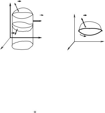
Proof. Let the domain G be bounded by the closed surface σ . Let this domain be bounded from below by a surface σ1 , defined by the equation z = z1 (x, y) ,

and from above it be bounded by a surface σ2 , defined by the equation z = z2 (x, y) ( z1 (x, y) ≤ z2 (x, y) ). Let this domain on each side be bounded by

the cylindrical surface		σ3	with generator			parallel to	the axis Oz. Let the
functions z1 (x, y) , z2 (x,		y)	be continuous in closed domain D being the projection
of the domain G on the plane Оху (Fig. 8.6).
Let’s consider triple integral
∫∫∫	∂R dxdydz = ∫∫ dxdy			z ( x, y)	∂R dz =∫∫ R(x, y, z)		z	2	( x, y)
				z ( x, y)			z		( x, y)
				1 ∫					dxdy =
G	∂z	D		z ( x, y)	∂z	D	z ( x, y)
				1				1
									187

http://vk.com/studentu_tk, http://studentu.tk/

= ∫∫ R(x, y, z2 (x,	y))dxdy −∫∫ R(x, y, z1 (x, y))dxdy.
D	D

We’ll replace the double integrals in the right part of equality by the surface integrals of the second type on the external side of surfaces σ2 and σ1 accordingly,

considering also angles between a normal n and the axis Оz. We’ll get

∫∫∫	∂R dxdydz = ∫∫ R(x, y, z)dxdy +∫∫ R(x, y, z)dxdy.
G	∂z	σ 2	σ1

As on the side σ3 , perpendicular to the plane Оху, equality ∫∫ Rdxdy = 0, is

fulfilled, then				σ 3
fulfilled, then
∫∫∫	∂R dxdydz = ∫∫ R(x, y, z)dxdy +∫∫ R(x, y, z)dxdy +
G	∂z	σ 2	σ1
G	+∫∫ R (x,	σ 2	σ1
	+∫∫ R (x,	y, z)dxdy = ∫∫ R (x,		y, z)dxdy.
	G		σ
Thus,		∂R dxdydz =
	∫∫∫	∂R dxdydz =	∫∫ R (x,	y, z)dxdy.	(8.4)
	G	∂z	σ
Similarly we’ll prove formulas
	∫∫∫	∂P dxdydz =	∫∫ P (x,	y, z)dydz,	(8.5)
	G	∂x	σ
	∫∫∫	∂Q dxdydz =	∫∫ Q[x,	y, z]dxdz.	(8.6)
	G	∂y	σ

Having added equalities (8.4) — (8.6) term by term, we’ll get the OstrogradskyGauss formula.

Remarks.

1.Ostrogradsky—Gauss Formula is convenient for using to calculate surface integrals on the closed surfaces.

2.Ostrogradsky—Gauss Formula is executed for the case when domain G may be divided into finite set of subdomains of the considered kind.

8.6. Stokes’ Formula

Stokes’ formula establishes connection between the surface and the line integrals.

188

http://vk.com/studentu_tk, http://studentu.tk/

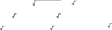
Theorem

If functions P(x, y, z) , Q(x, y, z) , R(x, y, z)

are continuous together

with the partial derivatives of the first order at the points of the

oriented surface σ , then Stokes’ formula is satisfied

∂Q

−

∂P

∂R

−

∂Q

∂P

−

∂R

∫∫

∂x

dxdy +

∂y

dydz +

dxdz =

∂y

∂z

∂x

= ∫ Pdx + Qdy + Rdz,

where L is the boundary of the surface σ and integration along the curve L is realized in positive direction concerning the selected side of a surface σ , i.e. from a normal corresponding to the selected side, detour of the contour L occurs counter-clockwise (Fig. 8.7).

z		n z = z2 (x, y)
		σ2
		n
		σ3
О	n	z =σ1z1 (x, y)
О	n	y
		y
		D

Fig. 8.6

Fig. 8.7

Remarks.

1.Stokes’ formula enables to evaluate line integrals of the second type on the closed contours by means of surface integrals.

2.From Stokes’ formula it follows, that if the equalities

∂Q	=	∂P	,	∂R	=	∂Q	,	∂P	=	∂R	,
∂x		∂y		∂y		∂z		∂z		∂x

are fulfilled, then line integral on any closed contour is equal to zero:

∫ Pdx + Qdy + Rdz = 0.

So, in this case the line integral does not depend on the form of integration way.

189

http://vk.com/studentu_tk, http://studentu.tk/

8.7.Some Applications of Surface Integrals

1.The area Sσ of the surface σ is calculated by formula

Sσ = ∫∫ dσ .

Compare this formula to the formula (6.13).

2. Mass m of the surfaces σ with the given surface density γ(x, y, z) at each point of the surfaces is calculated by formula

m = ∫∫ γ(x, y, z)dσ.

3. Coordinates xc ,

yc , zc of the centre of mass of a surface σ is defined by

formulas

x =

∫∫

xγ(x,

y, z)dσ,

y =

∫∫

yγ(x,

y, z)dσ,

(8.7)

∫∫

zc =

γ(x, y, z)dσ.

Micromodule 8

EXAMPLES OF PROBLEM SOLUTIONS

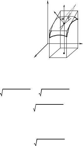
Example 1. Evaluate the surface integral of the first type I = ∫∫(x − 2z)dσ

over the part of the plane x + y + z = 1, placed in the first octant (Fig. 8.8). Solution. The surface σ is given by the equation z = 1− x − y, where function

z and its partial derivatives z′	= −1,	z′	= −1 are continuous in bounded closed
x		y

domain D being the projection of the surface σ on the plane Oху. Therefore the given integral exists. We’ll evaluate it accordingly to the formula (8.2):

I = ∫∫ (x − 2(1− x − y))				1+ (−1)2 + (−1)2 dxdy =								3∫∫ (−2 + 3x + 2 y)dxdy =
D													D
1	1− x								1									1− x
= 3∫ dx ∫ (−2 + 3x + 2y)dy = 3∫(−2y + 3xy + y2 )																			dx =
0	0								0									0
1		2			2			5		2			3		1				3	1	3
1		2			2			5		2			3		1				3	1	3
= 3∫(5x − 2 − 3x			+ (1	− x)		)dx =	3		x		− 2x − x			−		(1	− x)			= −		.
= 3∫(5x − 2 − 3x			+ (1	− x)		)dx =	3	2	x		− 2x − x			−	3	(1	− x)			= −	6	.
0								2							3					0	6

190

http://vk.com/studentu_tk, http://studentu.tk/

<<< < Предыдущая 1 2 3 4 5 6 7 8 9 10 11 12 13 14 15 16 17 1819 / 2419 20 21 22 23 24 > Следующая >>>

Соседние файлы в предмете [НЕСОРТИРОВАННОЕ]

#
19.02.20169 Mб96Higher_Mathematics_Part_1.pdf
#
19.02.20166.63 Mб1093Higher_Mathematics_Part_1.pdf
#
19.02.20169.73 Mб46Higher_Mathematics_Part_2.pdf
#
19.02.20167.48 Mб412Higher_Mathematics_Part_2.pdf
#
19.02.20167.31 Mб124Higher_Mathematics_Part_2.pdf
#
19.02.20169.11 Mб306Higher_Mathematics_Part_3.pdf
#
19.02.2016694.82 Кб14HiraganaKatakanaWorkSheet (1).pdf
#
11.09.2019192.23 Кб1hjuj;f.docx
#
27.11.2019386.05 Кб10How Airplanes Work.doc
#
03.01.2020126.46 Кб0HOW TO SOLVE GENETICS PROBLEMS.doc
#
20.11.201958.78 Кб9I exercise 5.docx