

Higher_Mathematics_Part_3
.pdf5.2. Definition and the Condition of the Existence
of a Double Integral
Let D be a bounded and closed domain and z = f (x, y) an arbitrary function
defined and bounded in this domain.We assume that the boundary of the domain D consists of a finite number of curves defined by equations y = f (x) or x = ϕ( y),
where f (x) and ϕ( y) are continuous functions.
Arbitrarily we divide the domain D into n parts Di which have no interior points in common and their areas are Si (I = 1, 2 … n).
In each subdomain Di |
we choose an arbitrary point Pi (ξi , ηi ). |
||||
We calculate a sum |
|
|
|
|
|
|
|
|
|
|
|
|
|
n |
|
|
|
|
σ = ∑ f (ξi , ηi ) |
Si , |
|
(5.6) |
|
|
|
i=1 |
|
|
|
which is the integral sum for the function |
f (x, y) |
in the domain D. |
|||
The diameter λ(D) |
of the domain D is the largest distance between the |
||||
boundary points of the domain. We denote the largest diameter of the subdomains Di by
|
λ = max λ(Di ) |
|
|
|
|
(5.7) |
||
|
|
1≤i≤ n |
|
|
|
|
|
|
|
|
|
|
|||||
Definition. If the integral sum (5.1) has a finite limit |
I as λ → 0, |
then this |
|
|||||
limit is called the double integral of the function |
f (x, |
y) |
over the domain D |
|
||||
and is denoted by one of the following symbols: |
|
|
|
|
|
|
||
|
|
|
|
|
|
|
|
|
|
n |
Si =∫∫ f (x, y)dS = ∫∫ f (x, |
|
|
|
|
||
|
I = lim ∑ f (ξi , ηi ) |
y)dxdy. |
|
(5.8) |
|
|||
|
λ →0 i=1 |
D |
D |
|
|
|
|
|
|
|
|
|
|
|
|
|
|
In this case the function f (x, y) is said to be integrable in the domain D, D is called the domain of integration, dS (or dxdy) is the element of the area.
Theorem (Sufficient condition). The function f (x, y) which is continuous
in a bounded closed domain D is integrable in this domain.
We must not assume, however, that a double integral exists only for continuous functions.
Remark. The volume of a cylindrical body is equal to the double integral of the function f (Pi ) = f (ξi , ηi ) over the domain D, i.e.
n |
Si = ∫∫ f (x, y)dxdy. |
|
V = lim ∑ f (ξi , ηi ) |
(5.9) |
|
λ →0 i=1 |
D |
|
|
|
101 |
http://vk.com/studentu_tk, http://studentu.tk/
Just as the problem of calculating the area of a curvilinear trapezoid leads to establishing the geometric meaning of the definite integral, the problem of calculating the volume of the body leads to the geometric interpretation of the double integral.
Remark. Mass of the plate is equal to the double integral of the function γ(x, y) over the domain D i. e.
|
|
n |
∫∫ γ(x, y)dxdy. |
|
|
||
|
m = lim |
∑γ(ξi , ηi ) Si = |
|
(5.10) |
|||
|
λ →0 |
i=1 |
D |
|
|
||
Remark. If f (x, y) = 1, (x, y) D , we obtain the area |
|
||||||
|
|
|
|
|
|
|
|
|
|
|
S = ∫∫ dxdy |
|
|
|
(5.11) |
|
|
|
D |
|
|
|
|
5.3. Principal Properties
The principal properties of the double integral are similar to the corresponding properties of the definite integral. So, we won’t prove them but only formulate these properties.
1. Linearity.
If the functions f (x, y) and g(x, y) are integrable over the domain D, and α and β are any real numbers, then the function αf (x, y) ± βg(x, y) is also integrable in D and
∫∫ |
|
∫∫ |
f (x, y)dxdy ± β |
∫∫ |
g (x, y)dxdy |
(5.12) |
|
|
αf (x, y) ± βg (x, y) dxdy = α |
|
|
|
|||
D |
|
|
D |
|
D |
|
|
2. |
If the function |
f (x, y) ≥ 0 over the domain D then |
|
|
|||
|
|
∫∫ f ( x, y )dxdy ≥ 0 |
|
|
(5.13) |
||
|
|
D |
|
|
|
|
|
3. |
If the functions |
f (x, y) ≥ g(x, |
y), and are integrable over a domain D then |
||||
|
∫∫ f (x, y)dxdy ≥ ∫∫ g (x, y)dxdy |
|
|
(5.14) |
|||
|
D |
D |
|
|
|
|
|
4. |
Additivity. |
|
|
|
|
|
|
If a domain D is the union of two domains D1 and D2, which have no internal points in common and in each of them the function f (x, y) is integrable, then
this function f (x, y) is also integrable in the domain D and
102
http://vk.com/studentu_tk, http://studentu.tk/
∫∫ f (x, |
y)dS =∫∫ f (x, |
y)dS + ∫∫ f (x, y)dS |
(5.15) |
D |
D1 |
D2 |
|
5. Estimation of integrals.
If the function f (x, y) is continuous in a closed bounded and m be respectively the largest and the smallest values of f ( be the area of D then
mS ≤ ∫∫ f (x, y)dxdy ≤ MS
domain D, let M x, y) in D, and S
(5.16)
D
6. If the function f (x, y) is continuous in a closed bounded domain D, then there exists at least one point P(x0, y0) D such as
∫∫ f (x, y)dS = f (x0 , y0 ) S, |
(5.17) |
|||
D |
|
|
|
|
where S is the area of D. |
1 |
|
|
|
Definition. The value f (x0 , y0 ) = |
∫∫ f (x, y)dxdy |
is known as the mean |
||
S |
||||
|
D |
|
||
value of f(x, y) in D.
We shall discuss now the calculation techniques of double integrals.
5.4. Reducing a Double Integral to an Iterated Integral
1. The case of a rectangular domain
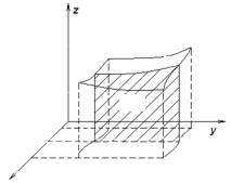
Let z = f (x, y), (x, y) D be nonnegative continuous
double integral of the function f (x, y) |
over the domain |
||||
volume of a cylindrical body V |
|
|
|
||
|
z |
||||
(Fig. 5.3) with the base D and |
|
|
|
||
|
|
|
|||
bounded from above by the surface |
|
|
|
||
z = f (x, y). |
Let’s |
find this volume |
|
|
|
V with the |
help |
of parallel-section |
|
M1 |
|
method, i.e. |
|
|
|
|
|
function then the D is equal to the
M2
b |
|
V = ∫ S(x)dx , |
(5.18) |
a
where S(x) is the area of a section perpendicular to the xy-plane. The
equations x = a, x = b define the planes bounding the given body.
|
|
|
S(x) |
|||
a |
C1 |
|
|
|
y |
|
|
|
|
||||
x |
|
|
|
|
||
D |
C2 |
|||||
|
||||||
b y = ϕ1(x) |
|
y = ϕ2(x) |
||||
|
|
|
||||
x
Fig. 5.3
103
http://vk.com/studentu_tk, http://studentu.tk/
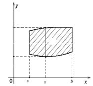
Let the domain D be bounded by continuous curves |
y = ϕ1 (x) and y = ϕ2 (x) |
||||||||
and x = a, x = b . Let ϕ1 (x) ≤ ϕ2 (x), |
x (a, b) |
(Fig. 5.4). |
|||||||
|
у |
|
|
|
С2 |
|
|
|
|
|
|
|
|
|
|
||||
|
|
|
|
|
|
|
|
|
|
у2 |
|
ϕ2(х) |
|
|
|||||
|
|
|
|
||||||
|
|
|
|
|
|
D |
|
|
|
у1 |
|
|
ϕ1(х) |
|
|
||||
|
С1 |
|
|
|
|||||
|
|
|
|
|
|
|
|
|
|
|
|
|
|
|
|
|
|
|
|
0 |
|
|
|
|
|
|
|
|
|
a |
x |
b |
x |
||||||
|
|
|
|
|
|
Fig. 5.4 |
|
|
|
|
|
|
|
|
|
|
|
|
|
We will draw a straight line across point (x; 0) which is parallel to Oy. This
line C1C2 intersects D only in two points. This domain is called a regular in a direction of an axis Oy.
Let’s consider a plane x = const, which is perpendicular to Ox, where x (a, b). The section of this plane with a cylindrical body is a curvilinear trapezoid C1M1M2C2 which bounds z = f (x, y), x = const, straight lines y = ϕ1(x), y = ϕ2 (x) and z = 0. The area of this trapezoid can be calculated as
|
|
|
y 2 |
|
ϕ2 ( x) |
|
||
|
S(x) = ∫ zdy = |
|
∫ |
|
f (x, y) dy. |
|||
|
|
|
y1 |
|
ϕ1 ( x) |
|
||
Substitution gives |
|
|
|
|
|
|
|
|
|
|
b |
|
b |
ϕ2 |
( x) |
|
|
|
V = |
∫ |
S(x)dx = |
∫ |
∫ |
|
|
|
|
|
|
|
|
f (x, y)dy dx. |
|||
|
|
a |
|
a ϕ1 ( x) |
|
|
||
Hence |
|
|
|
|
|
|
|
|
|
|
|
|
|
|
|
|
|
|
|
|
|
|
b |
ϕ2 |
( x) |
|
|
∫∫ f (x, y)dxdy = ∫ dx |
∫ f (x, y)dy. |
||||||
|
D |
|
|
|
a |
|
ϕ1 ( x) |
|
(5.19)
(5.20)
(5.21)
Definition. The relation is called iterated (or repeated) integrals of f (x, y) over the domain D.
104
http://vk.com/studentu_tk, http://studentu.tk/
Suppose the domain D is such that D is bounded by x = ψ1 ( y), x = ψ2 ( y)
and y = c, y = d, where ψ1(y) and ψ2 (y) are continuous functions, ψ1(y) ≤ ψ2 (y) for c ≤ y ≤ d (Fig. 5.5).
It is a regular domain in a direction of an axis Ox because any straight line,
which is parallel to Ox |
and passes |
through |
a point |
(0, y), intersects the |
||||||
boundary of the domain D not more than in two points. |
|
|||||||||
Then double integral can be written as |
|
|
|
|||||||
|
|
|
|
|
|
|
|
|
|
|
|
∫∫ f (x, |
|
|
|
d |
ϕ2 ( y) |
|
|
|
|
|
y)dxdy = ∫ dy ∫ f (x, |
y)dx |
|
(5.22) |
||||||
|
D |
|
|
|
c |
ϕ1 ( y) |
|
|
|
|
|
|
y |
|
|
|
|
||||
|
|
d |
|
|
|
|
||||
|
|
|
|
|
ψ1(y) |
D |
ψ2(y) |
|
||
|
|
|
|
|
C1 |
|
|
|
||
|
|
|
|
|
|
C2 |
|
|||
|
|
y |
|
|
||||||
|
|
c |
|
|
|
|
||||
|
|
|
|
|
x1 |
x2 |
x |
|||
|
|
|
|
|||||||
|
|
0 |
|
|
|
|||||
|
|
|
|
|
|
Fig. 5.5 |
|
|
|
|
|
|
|
|
|
|
|
|
|
||
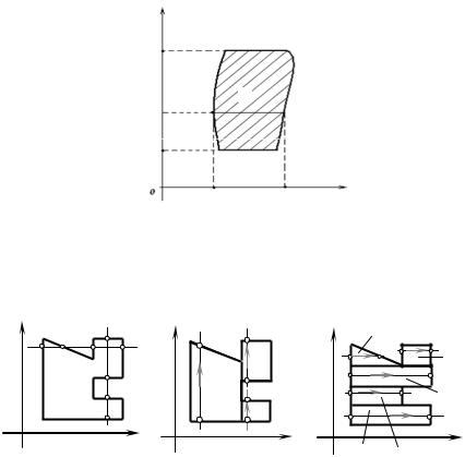
If the domain D isn’t regular, neither in the direction of the abscissa axis, nor ordinate axis (Fig. 5.6), then for the calculation of the double integral such domain should be divided into parts, which are regular at least in one direction. So, the division of the domain D shown in the Fig. 5.6.
y |
|
у |
|
у |
|
D4 |
|
|
|
|
|||
|
|
|
D2 |
|
|
D5 |
|
D |
|
D1 |
|
|
D3 |
|
|
|
D3 |
|
|
|
|
|
|
|
|
|
|
О |
x |
О |
x |
О |
D |
x |
|
|
|
|
|
1 |
D2 |
а |
|
b |
|
c |
|
|
|
|
|
Fig. 5.6 |
|
|
|
105
http://vk.com/studentu_tk, http://studentu.tk/
5.5. Change of Variables in Double Integral
5.5.1. Curvilinear Coordinates
Let function f (x, y) be defined in some closed and bounded domain D in xy-plane. Then there is I = ∫∫ f (x, y)dxdy .
D
Let, with the help of functions
x = x(u, v)
(5.23)
y = y(u, v)
in the given integral I, pass to the new variables u and v. Then in a domain D* in the uv-plane we are given (5.23) which we consider to be continuous and have continuous partial derivatives.
Suppose from (5.23), the functions
|
|
u = u(u, v) |
(5.24) |
|
|
v = v(u, v) |
|
can be found unequivocally. |
|
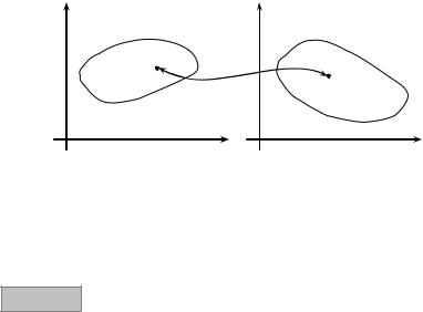
M (x, y) D ↔ |
|
So with formulas (5.22) and (5.23) we have for any point |
|||
↔ M * (u, v) D* |
(Fig.5.7). |
|
|
y |
|
y |
|
|
(x, y) |
|
|
|
D |
(u, v) |
|
|
|
|
|
|
|
D* |
|
O |
|
x O* |
u |
|
|
Fig. 5.7 |
|
It is said to be a one-to-one correspondence between two domains. Suppose the set of all points M * (u, v) form the bounded closed domain D*.
Formula (5.23) is called the formula of a transformation of coordinates. Formula (5.24) is called the formula for the inverse-transformation.
Theorem If the transformation (5.23) transfers the closed bounded domain D to the closed bounded domain D* by one-to-one and if
functions (5.23) have continuous partial derivatives of the first order and
106
http://vk.com/studentu_tk, http://studentu.tk/
|
∂x |
∂x |
|
|
|
|
|
||
I (u, v) = |
∂u |
∂v |
≠ 0. |
(5.25) |
|
∂y |
∂y |
|
|
|
∂u |
∂v |
|
|
|
|
|
|
|
in the domain D* and the function f(x, y) is continuous in the domain D, then the formula for a change of variables
∫∫ f (x, y)dxdy |
= ∫∫ f (x(u,v), y(u,v)) |
|
J (u, v) |
|
dudv |
(5.26) |
|
|
|||||
D |
D* |
|
||||
hold true.
Definition. The determinant (5.25) is Jacobs determinant or Jacobian.
The proof of the theorem is very complicated and is not given here. It should also be pointed out that formula (5.26) holds true in a more general case as well, in particular, Jacobian (5.25) can vanish at a finite number of points or curves.
Both in the double integral and in the definite integral a change of variables is the most important means of reducing it to a form more convenient for calculation.
5.5.2. Integral in Polar Coordinates
Let’s consider a polar system coordinates calculate Jacobian
|
∂x |
|
∂x |
|
= |
|
|
cos ϕ |
|
−ρ sin ϕ |
|
|
|
|
|
|
|
|
|
||||||
I (ρ, ϕ) = |
∂ρ |
|
∂ϕ |
|
|
|
|
|
||||
|
|
|
|
|||||||||
|
∂y |
|
∂y |
|
|
|
|
sin ϕ |
|
ρ cos ϕ |
|
|
|
∂ρ |
|
∂ϕ |
|
|
|
|
|
|
|
|
|
Considering that |
|
|
|
|
|
|
|
|
|
|
|
|
|
|
|
|
|
|
|
|
|
|
|
|
|
|
|
|
|
|
|
|
|
I (ρ, ϕ) |
|
= ρ, |
|
|
|
|
|
|
|
|
|
|
|
|
|||
|
|
|
|
|
|
|
|
|
|
|
|
|
x = ρ cos ϕ and y = ρ sin ϕ. We
= ρ cos2 ϕ + ρ sin2 ϕ = ρ .
(5.27)
the formula used to pass from an integral in rectangular coordinates to an integral on polar coordinates is:
∫∫ f (x, y)dxdy = ∫∫ f (ρ cos ϕ, ρ sin ϕ)ρdρdϕ. |
(5.28) |
|
D |
Dx |
|
If the domain D is bounded by straight lines, which in polar system with polar axis form angles α and β, α < β and curves ρ = ρ1 (ϕ), ρ = ρ2 (ϕ), ρ1 < ρ2
107
http://vk.com/studentu_tk, http://studentu.tk/
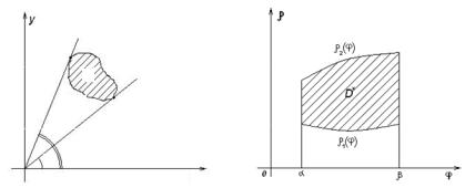
у |
|
|
|
ρ2(ϕ) |
у |
|
|
|
|
|
|||||
|
|
|
|
|
|||
|
|
|
|
|
|||
|
|
|
|
|
|
|
|
|
|
|
D |
|
|
|
|
|
|
|
ρ1(ϕ) |
|
|
|
|
|
|
α |
β |
|
|
|
|
|
|
|
|
х |
|
||
О |
|
|
|
||||
|
|
|
|
Fig. 5.8 |
Fig. 5.9 |
|
|
then the double integral is reduced to the iterated integral in a polar system |
|
||||||
|
|
|
|
|
|
|
|
|
|
|
|
∫∫ f (x, |
y)dxdy =∫αβ dϕ∫ρρ12((ϕϕ)) f (ρ cos ϕ, ρ sin ϕ)ρdρ. |
|
(5.29) |
|
|
|
|
D |
|
|
|
Remark. It is better to use polar coordinates if the domain D is a circle
x2 + y2 = R2 or ρ = R. |
Then the formula (5.28) can be written as |
||
|
|
|
|
|
|
2π |
R |
|
∫∫ f (x, y)dxdy = ∫ dϕ∫ f (ρ cos ϕ, ρ sin ϕ)ρdρ. |
||
|
D |
0 |
0 |
5.6.Application of Double Integrals
1.Volume of cylindrical body
As is known, the volume V of a curvilinear cylinder, which is bounded from above by the surface z = f(x, y) > 0, from below by the plane z = 0, and from the
lateral sides by a cylindrical surface whose generatrices are parallel to the z-axis and whose directrix is the contour of the domain D, can be found from the formula
|
V = ∫∫ f (x, y)dxdy, |
|
(5.30) |
|
D |
|
|
i.e. the volume of a body can be calculated by means of double integrals. |
|
||
2. Area of plane figures
We have established that the area S of the domain D can be calculated by means of the double integral from the formula
108
http://vk.com/studentu_tk, http://studentu.tk/
S = ∫∫ dxdy. |
(5.31) |
D |
|
This formula is more universal than the corresponding formula which expresses the area of a curvilinear trapezoid with the aid of a definite integral since the given formula is applicable not only to curvilinear trapezoids but also to figures whose position is arbitrary relative to the coordinate axes.
3. Surface area
Let the surface Q be defined by the equation z = f(x, y). The projection of Q on the xy-plane is the domain D and in this domain the function f(x, y) is
continuous and has continuous partial derivatives fx′ (x, y), |
fy′ (x, y), then |
||
|
Q = ∫∫ 1+ ( fx′ (x, y))2 + ( fy′ (x, y))2 dxdy. |
|
(5.32) |
|
D |
|
|
4. Mass of a planar figure
Suppose in xy-plane we have material plate, which has the form bounded by the domain D. At each point of D, density is defined as the continuous function
γ = γ(x, y), then
m = ∫∫ γ(x, y)dxdy. |
(5.33) |
D |
|
5. Coordinates of the center of mass of a plate
We seek the coordinates of the centre of mass of a plate which occupies a domain D in the xy-plane. Let γ(x, y) be the density of the plate at the point
M(x, y) ( γ(x, y) is a continuous function). The coordinates of the center of mass of the plate are defined by the formulas
x = |
∫∫ xγ(x, y)dxdy |
|
y = |
∫∫ yγ(x, y)dxdy |
|
|
D |
, |
D |
, |
(5.34) |
||
|
|
|||||
c |
m |
|
c |
m |
|
|
|
|
|
|
|
where m = ∫∫ γ(x, y)dxdy is the mass of the plate.
D
6. Static moment of inertia at a planar figure relative to coordinates axis
M y |
= ∫∫ xγ(x, |
y)dxdy, |
|
|
|
D |
|
(5.35) |
|
M x |
= ∫∫ yγ(x, |
y)dxdy. |
||
|
||||
|
D |
|
|
|
|
|
109 |
||
http://vk.com/studentu_tk, http://studentu.tk/

Then coordinates of the center of mass for the plate can be written as
x = |
M y |
, y = |
M |
x |
. |
(5.36) |
|
|
|
||||
c |
m |
c |
m |
|
||
|
|
|
||||
7. Moment of inertia
We know that the moment of inertia of a particle relative to an axis is equal to the product of the mass of the particle by the square of the distance from the particle to the axis, and the moment of inertia of a system of particles is equal to the sum of the moments of inertia of the particles.
Let the domain D of the xy-plane be occupied by a plate with a continuous density γ(x, y).
We have the following formula for the moment of inertia of the plate relative to the y-axis:
|
|
I y |
= ∫∫ x2 γ(x, |
y)dxdy. |
|
|
(5.37) |
|
|
|
D |
|
|
|
|
The moment of inertia of the plate relative to the x-axis: |
|
||||||
|
|
|
|
|
|
|
|
|
|
Ix |
= ∫∫ y2 γ(x, |
y)dxdy. |
|
|
(5.38) |
|
|
|
D |
|
|
|
|
The moment of inertia of the plate relative to the origin: |
|
||||||
|
|
|
|
||||
|
I0 = ∫∫(x2 + y2 )γ(x, y)dxdy, |
|
(5.39) |
||||
|
|
D |
|
|
|
|
|
i.e. I0 = Ix + Iy . |
|
|
|
|
|
||
Micromodule 5
EXAMPLES OF PROBLEM SOLUTIONS
Example 1. We calculate the double integral ∫∫(x + 2 y)dxdy over the domain
D
D = {(x, y) y = x2 , x = y2}.
Solution. Examine D. The parabolas |
y = x2 and x = y2 meet at the points |
||
Î (0, 0) |
and |
A(1, 1) (Fig. 5.10). So, x varies from 0 to 1, and ϕ (x) = x2 and |
|
|
|
|
1 |
ϕ2 (x) = |
x. |
Any straight line x = cost |
(0 ≤ x ≤ 1) crosses the boundary of the |
region at not more than two points. |
|
||
110 |
|
|
|
http://vk.com/studentu_tk, http://studentu.tk/