Higher_Mathematics_Part_3

6.2.21.x2 + y2 = 4 , z = 1, z = x + 2 y + 6 .

6.2.22.x2 + y2 = 9 , z = x2 + y2 + 4 , z = 0 .

6.2.23.x2 + z2 = 1, y = −1 , y = 10 − x2 − z2 .

6.2.24.x2 + y2 = 2x , z = 0 , z = x + y + 5 .

6.2.25.x2 + y2 = 4y , z = 0 , z = 2x + y + 6 .

Micromodule 7

BASIC THEORETICAL INFORMATION. LINE INTEGRALS

Line integrals of the first and second type. Properties and evaluation. Green’s formula. Conditions for a line integral being pathindependent. Integration of total differentials. Application.

Key words: a line integral of the first type — криволінійний інтеграл першого роду, smooth — гладкий, piecewise smooth — кусково-гладкий, path-independent — незалежний від шляху, simple connected — однозв’язний, doubly connected — двозв’язний, triply connected — тризв’язний, spatial — просторовий, directrix — напрямна, generatrix — твірна, homogeneous — однорідний.

Literature: [3, part 2, item 2.4], [9, part 10, § 3], [15, part 12, item 12.3], [16, part 15, § 1—4], [17, part 3, § 9—10].

151

http://vk.com/studentu_tk, http://studentu.tk/

7.1. Line Integrals of the First Type. Basic Concepts

A line integral is generalization of a definite integral in the case when any curve is a domain of integration.

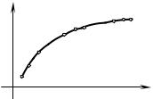
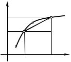
Let a smooth or piecewise smooth curve L bounded by points A and B (Fig. 7.1) be given in the plane Оху, and a continuous function z = f (x, y) be determined

on this curve. It should be reminded that a continuous curve x = x(t), y = y(t) is called smooth on a definite interval if functions x = x(t), y = y(t) have continuous, simultaneously not equal to zero derivatives x′(t) and y′(t) on this

interval. A continuous curve consisting of a finite number of smooth curves is called piecewise smooth.

Fig. 7.1

http://vk.com/studentu_tk, http://studentu.tk/

If the limit (7.1) exists, the function f (x, y) is called integrated over the

curve АВ, the curve АВ is a path or a contour of integration, the point A is called the initial point, and B is called the terminal point of the path of integration.

Theorem If a function f (x, y) is continuous over a smooth curve АВ then a line integral of the first type ∫ f (x, y)dl exists.

AB

Properties of a line integral of the first type are similar to corresponding properties of a definite integral (formulate them yourselves). However there is one property which essentially differs from the corresponding property of the definite integral.

The line integral of the first type does not de-

pend on the direction of integration over the con- z tour АВ, i.e.

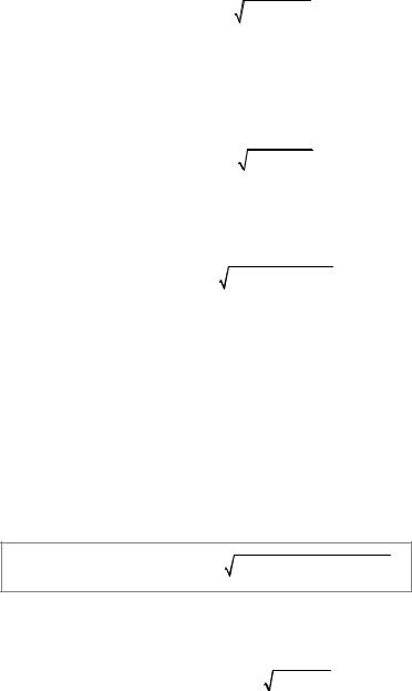
The geometrical significance of a line integral of the first type.

The line integral of the first type ∫ f (x, y)dl , where f (x, y) ≥ 0 ,

AB

numerically is equal to the area of a part of cylindrical surface whose directrix АВ lies in the plane Оху and generatrices are parallel to the axis Оz, provided

the cylindrical surface is bounded from above by the surface z = f (x, y) , from below by the plane Оху (Fig. 7.2).

7.2. Evaluation of a Line Integral of the First Type

Evaluation of a line integral of the first type is reduced to evaluation of a definite integral. We shall formulate rules of its evaluation in cases when the curve of integration is given by an explicit equation, in parametric form and in polar coordinates.

1. If the path АВ is given by the equation y = y(x) , x [а; b] (a is the

abscissa of the point A, b is the abscissa of the point В) where the functions y(x) and y′(x) are continuous in the segment [a; b], and the function f (x, y)

is continuous at each point of the path АВ, then

153

http://vk.com/studentu_tk, http://studentu.tk/

ordinate of the point A, d is the ordinate of the point В) where functions x( y)

where the value of the parameter α corresponds to the point A, and β to the point B and the function f (x, y) is continuous over the path АВ.

Remark. A line integral of the first type of a function f (x, y, z) over a

spatial curve АВ is defined analogously with a line integral of the first type of a function f (x, y) .

β

∫ f (x, y, z)dl = ∫ f (x(t), y(t), z(t)) (x′(t))2 + ( y′(t))2 + (z′(t))2 dt.

AB α

IІI. If a plane curve АВ is given by the equation ρ = ρ(ϕ) ( α ≤ ϕ ≤ β ) in polar coordinates, then

http://vk.com/studentu_tk, http://studentu.tk/

7.3. Line Integrals of the Second Type. Basic Concepts

Let functions of two variables P(x, y) and Q(x, y) be determined and

continuous at points of the arc АВ of a smooth curve L. Unlike integrals of the first type we shall consider a curve as a directed line, for which the points A and B are respectively initial and terminal points of the arc АВ. We break up the arc АВ into n arbitrary parts by points

А =A0, А1, А2, ..., Ап = В.

which depends neither on the way of splitting of the path АВ, nor on a choice of

Remark. A line integral

∫ P(x, y, z)dx + Q(x, y, z)dy + R(x, y, z)dz

L

over a spatial curve L is defined similarly.

155

http://vk.com/studentu_tk, http://studentu.tk/

∫ P(x, y, z)dx + Q(x, y, z)dy + R(x, y, z)dz,

α

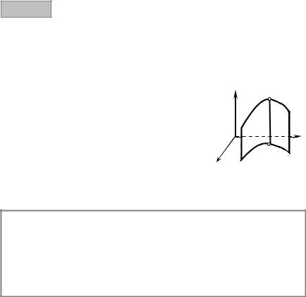
4. Let a contour of integration be a line segment lying in the plane Oxy and parallel to the axis Oy (Fig. 7.4, а). Then its equation is x = x0 , so dx = 0 . If to

а b

Fig. 7.4

If the contour of integration consists of some parts which have different equations, the integral is equal to the sum of the integrals evaluated for each part.

It follows from formulas (7.6) — (7.7) that a line integral of the second type has properties similar to properties of a definite integral. In particular, we must note that if a direction of integration is reversed the line integral of the second type changes the sign by opposite:

∫ P(x, y)dx + Q(x, y)dy = − ∫ P(x, y)dx + Q(x, y)dy,

AB BA

157

http://vk.com/studentu_tk, http://studentu.tk/

while the line integral of the first type does not depend on a direction of integration. Actually, with change of a direction of integration projections of a

vector Ai−1 Ai onto the axes Ox and Оу change their signs (Fig. 7.3).

If a curve of integration L is closed (Fig. 7.5) we get the line integral over the closed contour (or a contour integral) often designated as:

∫ Pdx + Qdy.

L

The value of the contour integral depends solely on the orientation of the contour, that is, on the direction of integration. The closed contour L is termed positively oriented if the contour is traced counter-clockwise, and if otherwise then negatively oriented.

where direction of integration along the contour L is positive (counterclockwise).

Proof. Let a domain D, called regular (Fig. 7.5), be bounded by a positively oriented contour L having at most two common points with every straight line parallel to the axis Ox or Oy. We can prove, that

158

http://vk.com/studentu_tk, http://studentu.tk/

Taking into account linearity of a line integral of the second type, the statement of the theorem turns to be true.

Remark. Green’s formula is valid for any domain which can be split into a finite number of regular domains.

7.6. Independence of a Line Integral of a Path of Integration

If a value of a line integral of the second type remains constant over all possible curves connecting initial and terminal points of integration, then the line integral is said to be independent of the form of a path of integration.

Let us remind the concept of simple and multiple connected domains.

A domain is said to be simple connected if it is bounded by one closed without points of self-intersection continuous piecewise smooth curve. So, shown on Fig. 7.6: a) is a simple connected domain; b) is a doubly connected domain; c) is a triply connected domain.

with their partial derivatives of the first order in a simply connected domain D. Then, for the line integral ∫ P(x, y)dx + Q(x, y)dy, to be

L

independent of the path of integration lying within the domain D it is necessary and sufficient that for all the points of the domain D the condition

should hold.

159

http://vk.com/studentu_tk, http://studentu.tk/

In conditions of this theorem the following statements are valid:

а) the expression under the integral sign is the total differential of a function u(x, y) , i.e.

P(x, y)dx + Q(x, y)dy = du(x, y) ;

b) ∫ P(x, y)dx + Q(x, y)dy = u(xB , yB ) − u(xA , yA ),

L

where A(xA , yA ) and B(xB , yB ) are initial and terminal points of the path of

integration;

c) the line integral taken round any closed contour L lying entirely within the domain D is equal to zero:

∫ P(x, y)dx + Q(x, y)dy = 0.

L

It is possible to prove that the statement of the theorem and the statements а) — c) are equivalent, i.e. each of them implies three others.

Let the condition ∂∂Py = ∂∂Qx be valid, then, after using Green’s formula (7.9), we receive

So, it follows from the theorem that the condition c) is fulfilled.

Let us assume, that the condition b) is fulfilled, i.e. the expression under the integral sign is the total differential of the function u(x, y) :

P(x, y)dx + Q(x, y) = du(x, y),

on the other hand, by definition of differential

http://vk.com/studentu_tk, http://studentu.tk/