aswath_damodaran-investment_philosophies_2012

R e l a t i v e V a l u e M o d e l s In relative value models, you examine how markets are priced relative to other markets and to fundamentals. How is this different from intrinsic value models? While the two approaches share some characteristics, this approach is less rigid insofar as it does not require that you work within the structure of a discounted cash flow model. Instead, you make comparisons either of markets over time (the S&P in 2012 versus the S&P in 1990) or of different markets at the same point in time (U.S. stocks in 2012 versus European stocks in 2012).

Comparisons across Time In its simplest form, you can compare the way stocks are priced today to the way they used to be priced in the past and draw conclusions on that basis. Thus, as we noted in the section on historic norms, many analysts argue that stocks today, priced at 13 times earnings in early 2012, are cheap because stocks historically have been priced at 15 to 16 times earnings.

While reversion to historic norms remains a very strong force in financial markets, we should be cautious about drawing too strong a conclusion from such comparisons. As the fundamentals (interest rates, risk premiums, expected growth, and payout) change over time, the P/E ratio will also change. Other things remaining equal, for instance, we would expect the following.

An increase in interest rates should result in a higher cost of equity for the market and a lower P/E ratio.

A greater willingness to take risk on the part of investors will result in a lower risk premium for equity and a higher P/E ratio across all stocks.

An increase in expected growth in earnings across firms will result in a higher P/E ratio for the market.

In other words, it is difficult to draw conclusions about P/E ratios without looking at these fundamentals. A more appropriate comparison is therefore not between P/E ratios across time, but between the actual P/E ratio and the predicted P/E ratio based on fundamentals existing at that time.

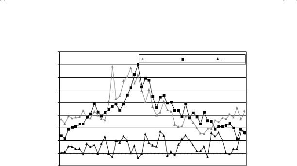
Figure 12.6 summarizes the earnings/price ratios (or earnings yield) for S&P 500, Treasury bond rates, and the difference between bond and bill rates at the end of each year from 1960 to 2010.

You do not need to be a statistician to note that earnings-to-price ratios are high (and P/E ratios are low) when the Treasury bond rates are high, and the earnings-to-price ratios decline when Treasury bond rates drop. This strong positive relationship between E/P ratios and T-bond rates is evidenced by the correlation of 0.69 between the two variables. In addition, there is evidence that the term structure also affects the E/P ratio. In the following

Based on this regression, we can predict the E/P ratio for the S&P 500 in November 2011, with the T-bill rate at 0.2 percent and the T-bond rate at 2.2 percent.

E/P2011 = 0.0266 + 0.6746(0.022) − 0.3131(0.022 − 0.02) = 0.0408 or 4.08%

N U M B E R W A T C H

Relative value of S&P 500 index: Take a look at the most recent relative valuation of the S&P 500.

Since the S&P 500 was trading at a multiple of 15 times earnings in November 2011, this would have indicated a significantly undervalued market. This regression can be enriched by adding other variables (which should be correlated to the price-earnings ratio), such as expected growth in GDP and payout ratios, as independent variables. The biggest uncertainty is whether the multiple market crises from 2008 to 2011 have rendered historical relationships between P/E ratios and interest rates meaningless, at least for the United States.

Comparisons across Markets Comparisons are often made between priceearnings ratios in different countries with the intention of finding undervalued and overvalued markets. Markets with lower P/E ratios are viewed as undervalued, and those with higher P/E ratios are considered overvalued. Given the wide differences that exist between countries on fundamentals, it is clearly misleading to draw these conclusions. For instance, you would expect to see the following, other things remaining equal:

Countries with higher real interest rates should have lower P/E ratios than countries with lower real interest rates.

Countries with higher expected real growth should have higher P/E ratios than countries with lower real growth.

Countries that are viewed as riskier (and thus command higher risk premiums) should have lower P/E ratios than safer countries.

Countries where companies are more efficient in their investments (and earn a higher return on these investments) should trade at higher P/E ratios.

We will illustrate this process to compare P/E ratios across markets. Table 12.7 summarizes P/E ratios across different developed markets in July 2000, together with dividend yields and interest rates (short term and long term) at the time.

A naive comparison of P/E ratios suggests that Japanese stocks, with a P/E ratio of 52.25, are overvalued, while Belgian stocks, with a P/E ratio of 14.74, are undervalued. There is, however, a strong negative correlation between P/E ratios and 10-year interest rates (–0.73) and a positive correlation between the P/E ratio and the yield spread (0.70). A cross-sectional regression of the P/E ratio on interest rates and expected growth yields the following.

P/E ratio = 42.62 − 360.9 (10-year rate) + 846.6(10-year rate − 2-year rate) [2.78] [−1.42] [1.08] R2 = 59%

The coefficients are of marginal significance, partly because of the small size of the sample. Based on this regression, the predicted P/E ratios for the countries are shown in Table 12.8.

From this comparison, Belgian and Swiss stocks would be the most undervalued, while U.S. stocks would be the most overvalued.

T A B L E 1 2 . 7 P/E Ratios for Developed Markets, July 2000

Interest rates: Short-term interest rates in these countries.

D e t e r m i n a n t s o f S u c c e s s

Can you time markets by comparing stock prices now to prices in the past or to how stocks are priced in other markets? Though you can make judgments about market underor overvaluation with these comparisons, there are two problems with this analysis.

1.Since you are basing your analysis by looking at the past, you are assuming that there has not been a significant shift in the underlying relationship. Structural or permanent shifts wreak havoc on these models.

2.Even if you assume that the past is prologue and that there will be reversion back to historic norms, you do not control this part of the process. In other words, you may find stocks to be overvalued on a relative basis, but they become more overvalued over time. Thus convergence is neither timed nor even guaranteed.

How can you improve your odds of success? First, you can try to incorporate into your analysis those variables that reflect the shifts that you believe have occurred in markets. For instance, if you believe that the influx of hedge fund money into the equity markets over the past two decades has changed the fundamental pricing relationship, you can include the percentage

of stock held by hedge funds in your regression. Second, you can have a longer time horizon, since you improve your odds on convergence.

T H E I N F O R M A T I O N L A G W I T H F U N D A M E N T A L S

If you are considering timing the market using macroeconomic variables such as inflation or economic growth, you should also take into account the time lag before you will get this information. Consider, for instance, a study that shows that there is high positive correlation between GDP growth in a quarter and the stock market’s performance in the next. An obvious strategy would be to buy stocks after a quarter of high GDP growth and sell after a quarter of negative or low GDP growth. The problem with the strategy is that the information on GDP growth will not be available to you until you are two months into the next quarter.

If you use a market variable such as the level of interest rates or the slope of the yield curve to make your market forecasts, you are in better shape since this information should be available to you contemporaneously with the stock market. In building these models, you should be careful and ensure that you are not building a model where you will have to forecast interest rates in order to forecast the stock market. To test for a link between the level of interest rates and stock market movements, you would look at the correlation between interest rates at the beginning of each year and stock returns over the year. Since you can observe the former before you make your investment decision, you would have the basis for a viable strategy if you find a correlation between the two. If you had run the test between the level of interest rates at the end of each year and stock returns during the year, implementing an investment strategy even if you find a correlation would be problematic since you would have to forecast the level of interest rates first.

T H E E V I D E N C E O N M A R K E T T I M I N G

While we have looked at a variety of ways in which investors try to time markets from technical indicators to fundamentals, we have not asked a more fundamental question: Do those who claim to time markets actually succeed? In this section, we consider a broad range of investors who try to time markets and examine whether they succeed.

funds decreased dramatically in 2008, largely in reaction to the market drop in that year.

The question of whether mutual funds are successful at market timing has been examined widely in the literature going back four decades. A study in 1966 by Treynor and Mazuy suggested that we look at whether the betas of funds increase when the market return is large in absolute terms by running a regression of the returns on a fund against both market and squared market returns:24

RFund, Period t = a + b ReturnMarket, t + c ReturnMarket, t2

If a fund manager has significant market timing abilities, they argued, the coefficient c on squared returns should be positive. This approach, when tested out on actual mutual fund returns, yields negative values for the coefficient on squared returns, indicating negative market timing abilities rather than positive ones. In 1981, Merton and Henrikkson modified this equation to consider whether funds earned higher returns in periods when the market was positive, and found little evidence of market timing as well.25

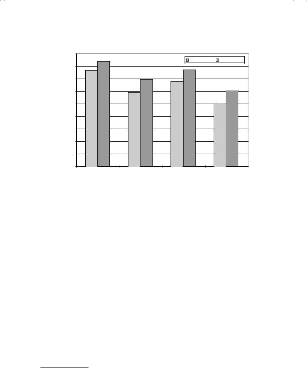
T a c t i c a l A s s e t A l l o c a t i o n a n d O t h e r M a r k e t T i m i n g F u n d s In the aftermath of the crash of 1987, a number of mutual funds sprang up claiming that they could have saved investors the losses from the crash by steering them out of equity markets prior to the crash. These funds were called tactical asset allocation funds and made no attempt to pick stocks. Instead, they argued that they could move funds between stocks, Treasury bonds, and Treasury bills in advance of major market movements and allow investors to earn high returns. Since 1987, though, the returns delivered by these funds have fallen well short of their promises. Figure 12.8 compares the returns on a dozen large tactical asset allocation funds over 5-year and 10-year periods (1989–1998) to the overall market as well as to fixed mixes—50 percent in both stocks and bonds, and 75 percent stocks/25 percent bonds. We call the last two couch potato mixes, reflecting the fact that we are making no attempt to time the market. The tactical asset allocation funds under perform the overall market and the couch potato funds.

24Jack L. Treynor and Kay Mazuy, “Can Mutual Funds Outguess the Market?”

Harvard Business Review 44 (1966): 131–136.

25Roy D. Henriksson and Robert C. Merton, “On Market Timing and Investment Performance, II: Statistical Procedures for Evaluating Forecasting Skills,” Journal of Business 54 (1981): 513–533.