aswath_damodaran-investment_philosophies_2012

ignore transaction costs on both buying stock and selling short on stocks. Third, we assume that the dividends paid on the stocks in the index are known with certainty at the start of the period. If these assumptions are unrealistic, the index futures arbitrage will be feasible only if prices fall outside a band, the size of which will depend on the seriousness of the violations in the assumptions.

Thus, if we assume that investors can borrow money at rb and lend money at ra and that the transaction cost of buying stock is tc and selling short is ts, the band within which the futures price must stay can be written as:

(S − ts ) (1 + ra − y)t F (S + tc) (1 + rb − y)t

The arbitrage that is possible if the futures price strays outside this band is illustrated in Figure 11.4.

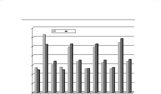
In practice, one of the issues that you have to factor in is the seasonality of dividends since the dividends paid by stocks tend to be higher in some months than others. Figure 11.5 graphs out cumulative dividends paid by stocks in the S&P 500 index on U.S. stocks in 2009 and 2010 by month of the year.

Thus, dividend yields seem to peak in February, May, August, and November in both years. An index futures contract coming due in these months is much more likely to be affected by dividends, especially as maturity draws closer.

Treasury Bond Futures The Treasury bond futures traded on the Chicago Board of Trade (CBOT) require the delivery of any government bond with a maturity greater than 15 years, with a no-call feature for at least the first 15 years. Since bonds of different maturities and coupons will have different prices, the CBOT has a procedure for adjusting the price of the bond for its characteristics. The conversion factor itself is fairly simple to compute and is based on the value of the bond on the first day of the delivery month, with the assumption that the interest rate for all maturities equals a preset rate per annum (with semiannual compounding). For instance, if the preset rate is 8 percent, you can compute the conversion factor for a 9 percent coupon bond with 18 years to maturity. Working in terms of a $100 face value of the bond, the value of the bond can be written as follows, using the interest rate of 8 percent.

Source: Bloomberg.

The conversion factor for this bond is 111.55. Generally, the conversion factor will increase as the coupon rate increases and with the maturity of the delivered bond.

This feature of Treasury bond futures (i.e., that any one of a menu of Treasury bonds can be delivered to fulfill the obligation on the bond) provides an advantage to the seller of the futures contract. Naturally, the cheapest bond on the menu, after adjusting for the conversion factor, will be delivered. This delivery option has to be priced into the futures contract. There is an additional option embedded in Treasury bond futures contracts that arises from the fact that the seller does not have to notify the clearinghouse until 8 p.m. about his intention to deliver. If bond prices decline after the close of the futures market, the seller can notify the clearinghouse of his intention to deliver the cheapest bond that day. If not, the seller can wait for the next day. This option is called the wild card option.

The valuation of a Treasury bond futures contract follows the same lines as the valuation of a stock index future, with the coupons of the Treasury bond replacing the dividend yield of the stock index. The theoretical value of a futures contract should be:

F = (S − PVC) (1 + r)t

where F* = Theoretical futures price for Treasury bond futures contract

S = Spot price of Treasury bond

PVC = Present value of coupons during life of futures contract r = Risk-free interest rate corresponding to futures life

t = Life of futures contract

If the futures price deviates from this theoretical price, there should be the opportunity for arbitrage. These arbitrage opportunities are illustrated in Figure 11.6.

This valuation ignores the two options described earlier—the option to deliver the cheapest-to-deliver bond and the option to have a wild card play. These give an advantage to the seller of the futures contract and should be priced into the futures contract. One way to build this into the valuation is to use the cheapest deliverable bond to calculate both the current spot price and the present value of the coupons. Once the futures price is estimated, it can be divided by the conversion factor to arrive at the standardized futures price.

Currency Futures In a currency futures contract, you enter into a contract to buy a foreign currency at a price fixed today. To see how spot and futures currency prices are related, note that holding the foreign currency enables the investor to earn the risk-free interest rate (Rf) prevailing in that country while the domestic currency earns the domestic risk-free rate (Rd). Since investors can buy currency at spot rates, and assuming that there are no restrictions on investing at the risk-free rate, we can derive the relationship between the spot and futures prices. Interest rate parity relates the differential between futures and spot prices to interest rates in the domestic and foreign market.

where futures priced,f is the number of units of the domestic currency that will be received for a unit of the foreign currency in a forward contract, and spot priced,f is the number of units of the domestic currency that will be received for a unit of the same foreign currency in a spot contract. For instance, assume that the one-year interest rate in the United States is 2 percent and the one-year interest rate in Switzerland is 1 percent. Furthermore, assume that the spot exchange rate is $1.10 per Swiss Franc. The one-year futures price, based on interest rate parity, should be as follows:

Futures price$,Sfr = (1.02) $1.10 (1.01)

This results in a futures price of $1.1109 per Swiss franc.

If the futures price were lower than $1.1109, the actions would be reversed, with the same final conclusion. Investors would be able to take no risk, invest no money, and still end up with a positive cash flow at expiration. In the second arbitrage of Table 11.1, we lay out the actions that would lead to a riskless profit of 0.0054 Sfr.

S p e c i a l F e a t u r e s o f F u t u r e s M a r k e t s There are two special features of futures markets that can make arbitrage tricky. The first is the existence of margins. While we assumed when constructing the arbitrage that buying and selling futures contracts would create no cash flows at the time of the transaction, you have to put up a portion of the futures contract price (about 5 percent to 10 percent) as a margin in the real world. To compound the problem, this margin is recomputed every day based on futures prices that day (this process is called marking to market) and you may be required to come up with more margin if the price moves against you (down if you are a buyer, and up if you are a seller). If this margin call is not met, your position can be liquidated and you may never get to see your arbitrage profits.

N U M B E R W A T C H

Price limits and contract specifications: Take a look at the price limits and contract specifications on widely traded futures contracts.

The second feature is that the futures exchanges generally impose price movement limits on most futures contracts. If the price of the contract drops or increases by the amount of the price limit, trading is generally suspended for the day, though the exchange reserves the discretion to reopen trading in the contract later in the day. The rationale for introducing price limits is to prevent panic buying and selling on an asset based on faulty information or rumors, and to prevent overreaction to real information. By allowing investors more time to react to extreme information, it is argued, the price reaction will be more rational and reasoned. In the process, though, you can create a disconnect between the spot markets, where no price limits exist, and the futures markets, where they do.

F e a s i b i l i t y o f A r b i t r a g e a n d P o t e n t i a l f o r S u c c e s s If futures arbitrage is so simple, you may ask, how in a reasonably efficient market would arbitrage opportunities even exist? In the commodity futures market, for instance, Garbade and Silber find little evidence of arbitrage opportunities, and their

findings are echoed in other studies.1 In the financial futures markets, there is evidence that indicates that arbitrage is indeed feasible but only to a subset of investors. Differences in transaction costs seem to explain most of the differences. Large institutional investors, with close to zero transaction costs and instantaneous access to both the underlying asset and futures markets, may be able to find arbitrage opportunities where most individual investors would not. In addition, these investors are also more likely to meet the requirements for arbitrage—being able to borrow at rates close to the riskless rate and sell short on the underlying asset.

Note, though, that the returns are small even to these large investors and that arbitrage will not be a reliable source of profits, unless you can establish a competitive advantage on one of three dimensions.2 First, you can try to establish a transaction cost advantage over other investors, which will be difficult to do since you are competing with other large institutional investors. Second, you may be able to develop an information advantage over other investors by having access to information earlier than others. However, much of the information is pricing information and is public. Third, you may find a quirk in the data or pricing of a particular futures contract before others learn about it. As a consequence, the arbitrage possibilities seem to be greater when futures contracts are first introduced on an asset, since investors take time to understand the details of futures pricing. For instance, it took investors a while to learn to incorporate the effect of uneven dividends into stock index futures and the wild card option into Treasury bond futures. Presumably, investors who learned faster than the market would have been able to take advantage of the mispricing of futures contracts in these early periods and earn excess returns.

O p t i o n s A r b i t r a g e

As derivative securities, options differ from futures in a very important respect. They represent rights rather than obligations; calls give you the right to buy, and puts give you the right to sell. Consequently, a key feature of options is that the losses on an option position are limited to what you paid for the option, if you are a buyer. Since there is usually an underlying asset that is traded, you can, as with futures contracts, construct positions that essentially are risk-free by combining options with the underlying asset.

1K. D. Garbade and W. L. Silber, “Price Movements and Price Discovery in Futures and Cash Markets,” Review of Economics and Statistics 115 (1983): 289–297.

2A study of 835 index arbitrage trades on the S&P 500 futures contracts estimated that the average gross profit from such trades was only 0.30 percent.