

Robert I. Kabacoff - R in action
.pdf16 |
CHAPTER 1 Introduction to R |
R comes with a standard set of packages (including base, datasets, utils, grDevices, graphics, stats, and methods). They provide a wide range of functions and datasets that are available by default. Other packages are available for download and installation. Once installed, they have to be loaded into the session in order to be used. The command search() tells you which packages are loaded and ready to use.
1.4.2Installing a package
There are a number of R functions that let you manipulate packages. To install a package for the first time, use the install.packages() command. For example, install.packages() without options brings up a list of CRAN mirror sites. Once you select a site, you’ll be presented with a list of all available packages. Selecting one will download and install it. If you know what package you want to install, you can do so directly by providing it as an argument to the function. For example, the gclus package contains functions for creating enhanced scatter plots. You can download and install the package with the command install.packages("gclus").
You only need to install a package once. But like any software, packages are often updated by their authors. Use the command update.packages() to update any packages that you’ve installed. To see details on your packages, you can use the installed.packages() command. It lists the packages you have, along with their version numbers, dependencies, and other information.
1.4.3Loading a package
Installing a package downloads it from a CRAN mirror site and places it in your library. To use it in an R session, you need to load the package using the library() command. For example, to use the packaged gclus issue the command library(gclus). Of course, you must have installed a package before you can load it. You’ll only have to load the package once within a given session. If desired, you can customize your startup environment to automatically load the packages you use most often. Customizing your startup is covered in appendix B.
1.4.4Learning about a package
When you load a package, a new set of functions and datasets becomes available. Small illustrative datasets are provided along with sample code, allowing you to try out the new functionalities. The help system contains a description of each function (along with examples), and information on each dataset included. Entering help(package="package_name") provides a brief description of the package and an index of the functions and datasets included. Using help() with any of these function or dataset names will provide further details. The same information can be downloaded as a PDF manual from CRAN.

Batch processing |
17 |
Common mistakes in R programming
There are some common mistakes made frequently by both beginning and experienced R programmers. If your program generates an error, be sure the check for the following:
■Using the wrong case—help(), Help(), and HELP() are three different functions (only the first will work).
■Forgetting to use quote marks when they’re needed—install.packages- ("gclus") works, whereas install.packages(gclus) generates an error.
■Forgetting to include the parentheses in a function call—for example, help() rather than help. Even if there are no options, you still need the ().
■Using the \ in a pathname on Windows—R sees the backslash character as an escape character. setwd("c:\mydata") generates an error. Use setwd("c:/mydata") or setwd("c:\\mydata") instead.
■Using a function from a package that’s not loaded—The function order. clusters() is contained in the gclus package. If you tr y to use it before loading the package, you’ll get an error.
The error messages in R can be cr yptic, but if you’re careful to follow these points, you should avoid seeing many of them.
1.5Batch processing
Most of the time, you’ll be running R interactively, entering commands at the command prompt and seeing the results of each statement as it’s processed. Occasionally, you may want to run an R program in a repeated, standard, and possibly unattended fashion. For example, you may need to generate the same report once a month. You can write your program in R and run it in batch mode.
How you run R in batch mode depends on your operating system. On Linux or Mac OS X systems, you can use the following command in a terminal window:
R CMD BATCH options infile outfile
where infile is the name of the file containing R code to be executed, outfile is the name of the file receiving the output, and options lists options that control execution. By convention, infile is given the extension .R and outfile is given extension
.Rout.
For Windows, use
"C:\Program Files\R\R-2.13.0\bin\R.exe" CMD BATCH--vanilla --slave "c:\my projects\myscript.R"
adjusting the paths to match the location of your R.exe binary and your script file. For additional details on how to invoke R, including the use of command-line options, see the “Introduction to R” documentation available from CRAN (http://cran.r-project.org).
18 |
CHAPTER 1 Introduction to R |
1.6Using output as input—reusing results
One of the most useful design features of R is that the output of analyses can easily be saved and used as input to additional analyses. Let’s walk through an example, using one of the datasets that comes pre-installed with R. If you don’t understand the statistics involved, don’t worry. We’re focusing on the general principle here.
First, run a simple linear regression predicting miles per gallon (mpg) from car weight (wt), using the automotive dataset mtcars. This is accomplished with the function call:
lm(mpg~wt, data=mtcars)
The results are displayed on the screen and no information is saved.
Next, run the regression, but store the results in an object:
lmfit <- lm(mpg~wt, data=mtcars)
The assignment has created a list object called lmfit that contains extensive information from the analysis (including the predicted values, residuals, regression coefficients, and more). Although no output has been sent to the screen, the results can be both displayed and manipulated further.
Typing summary(lmfit) displays a summary of the results, and plot(lmfit) produces diagnostic plots. The statement cook<-cooks.distance(lmfit) generates influence statistics and plot(cook) graphs them. To predict miles per gallon from car weight in a new set of data, you’d use predict(lmfit, mynewdata).
To see what a function returns, look at the Value section of the online help for that function. Here you’d look at help(lm) or ?lm. This tells you what’s saved when you assign the results of that function to an object.
1.7Working with large datasets
Programmers frequently ask me if R can handle large data problems. Typically, they work with massive amounts of data gathered from web research, climatology, or genetics. Because R holds objects in memory, you’re typically limited by the amount of RAM available. For example, on my 5-year-old Windows PC with 2 GB of RAM, I can easily handle datasets with 10 million elements (100 variables by 100,000 observations). On an iMac with 4 GB of RAM, I can usually handle 100 million elements without difficulty.
But there are two issues to consider: the size of the dataset and the statistical methods that will be applied. R can handle data analysis problems in the gigabyte to terabyte range, but specialized procedures are required. The management and analysis of very large datasets is discussed in appendix G.
1.8Working through an example
We’ll finish this chapter with an example that ties many of these ideas together. Here’s the task:
1Open the general help and look at the “Introduction to R” section.
2Install the vcd package (a package for visualizing categorical data that we’ll be using in chapter 11).
Working through an example |
19 |
3List the functions and datasets available in this package.
4Load the package and read the description of the dataset Arthritis.
5Print out the Arthritis dataset (entering the name of an object will list it).
6Run the example that comes with the Arthritis dataset. Don’t worry if you don’t understand the results. It basically shows that arthritis patients receiving treatment improved much more than patients receiving a placebo.
7Quit.
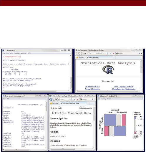
The code required is provided in the following listing, with a sample of the results displayed in figure 1.7.
Listing 1.3 Working with a new package
help.start()
install.packages("vcd")
help(package="vcd")
library(vcd)
help(Arthritis) Arthritis example(Arthritis) q()
Figure 1.7 Output from listing 1.3 including (left to right) output from the arthritis example, general help, information on the vcd package, information on the Arthritis dataset, and a graph displaying the relationship between arthritis treatment and outcome
20 |
CHAPTER 1 Introduction to R |
As this short exercise demonstrates, you can accomplish a great deal with a small amount of code.
1.9Summary
In this chapter, we looked at some of the strengths that make R an attractive option for students, researchers, statisticians, and data analysts trying to understand the meaning of their data. We walked through the program’s installation and talked about how to enhance R’s capabilities by downloading additional packages. We explored the basic interface, running programs interactively and in batches, and produced a few sample graphs. You also learned how to save your work to both text and graphic files. Because R can be a complex program, we spent some time looking at how to access the extensive help that’s available. We hope you’re getting a sense of how powerful this freely available software can be.
Now that you have R up and running, it’s time to get your data into the mix. In the next chapter, we’ll look at the types of data R can handle and how to import them into R from text files, other programs, and database management systems.

Creating2a dataset
This chapter covers
■Exploring R data structures
■Using data entr y
■Impor ting data
■Annotating datasets
The first step in any data analysis is the creation of a dataset containing the information to be studied, in a format that meets your needs. In R, this task involves the following:
■Selecting a data structure to hold your data
■Entering or importing your data into the data structure
The first part of this chapter (sections 2.1–2.2) describes the wealth of structures that R can use for holding data. In particular, section 2.2 describes vectors, factors, matrices, data frames, and lists. Familiarizing yourself with these structures (and the notation used to access elements within them) will help you tremendously in understanding how R works. You might want to take your time working through this section.
The second part of this chapter (section 2.3) covers the many methods available for importing data into R. Data can be entered manually, or imported from an
21

22 |
CHAPTER 2 Creating a dataset |
external source. These data sources can include text files, spreadsheets, statistical packages, and database management systems. For example, the data that I work with typically comes from SQL databases. On occasion, though, I receive data from legacy DOS systems, and from current SAS and SPSS databases. It’s likely that you’ll only have to use one or two of the methods described in this section, so feel free to choose those that fit your situation.
Once a dataset is created, you’ll typically annotate it, adding descriptive labels for variables and variable codes. The third portion of this chapter (section 2.4) looks at annotating datasets and reviews some useful functions for working with datasets (section 2.5). Let’s start with the basics.
2.1Understanding datasets
A dataset is usually a rectangular array of data with rows representing observations and columns representing variables. Table 2.1 provides an example of a hypothetical patient dataset.
Table 2.1 A patient dataset
PatientID |
AdmDate |
Age |
Diabetes |
Status |
|
|
|
|
|
1 |
10/15/2009 |
25 |
Type1 |
Poor |
2 |
11/01/2009 |
34 |
Type2 |
Improved |
3 |
10/21/2009 |
28 |
Type1 |
Excellent |
4 |
10/28/2009 |
52 |
Type1 |
Poor |
|
|
|
|
|
Different traditions have different names for the rows and columns of a dataset. Statisticians refer to them as observations and variables, database analysts call them records and fields, and those from the data mining/machine learning disciplines call them examples and attributes. We’ll use the terms observations and variables throughout this book.
You can distinguish between the structure of the dataset (in this case a rectangular array) and the contents or data types included. In the dataset shown in table 2.1, PatientID is a row or case identifier, AdmDate is a date variable, Age is a continuous variable, Diabetes is a nominal variable, and Status is an ordinal variable.
R contains a wide variety of structures for holding data, including scalars, vectors, arrays, data frames, and lists. Table 2.1 corresponds to a data frame in R. This diversity of structures provides the R language with a great deal of flexibility in dealing with data.
The data types or modes that R can handle include numeric, character, logical (TRUE/FALSE), complex (imaginary numbers), and raw (bytes). In R, PatientID, AdmDate, and Age would be numeric variables, whereas Diabetes and Status would be character variables. Additionally, you’ll need to tell R that PatientID is a case identifier, that AdmDate contains dates, and that Diabetes and Status are nominal
Data structures |
23 |
and ordinal variables, respectively. R refers to case identifiers as rownames and categorical variables (nominal, ordinal) as factors. We’ll cover each of these in the next section. You’ll learn about dates in chapter 3.
2.2Data structures
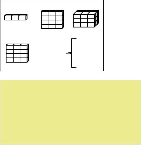
R has a wide variety of objects for holding data, including scalars, vectors, matrices, arrays, data frames, and lists. They differ in terms of the type of data they can hold, how they’re created, their structural complexity, and the notation used to identify and access individual elements. Figure 2.1 shows a diagram of these data structures.
Let’s look at each structure in turn, starting with vectors.
(b) Matrix |
(c) Array |
|
(a) Vector |
|
|
(d) Data frame |
|
|
|
Vectors |
|
(e) List |
Arrays |
|
Data frames |
|
|
|
|
|
|
Lists |
|
Columns can be different modes |
Figure 2.1 |
R data |
|
structures |
|
Some definitions
There are several terms that are idiosyncratic to R, and thus confusing to new users.
In R, an object is anything that can be assigned to a variable. This includes constants, data structures, functions, and even graphs. Objects have a mode (which describes how the object is stored) and a class (which tells generic functions like print how to handle it).
A data frame is a structure in R that holds data and is similar to the datasets found in standard statistical packages (for example, SAS, SPSS, and Stata). The columns are variables and the rows are obser vations. You can have variables of different types (for example, numeric, character) in the same data frame. Data frames are the main structures you’ll use to store datasets.
(continued)

24 |
CHAPTER 2 Creating a dataset |
Factors are nominal or ordinal variables. They’re stored and treated specially in R. You’ll learn about factors in section 2.2.5.
Most other terms should be familiar to you and follow the terminology used in statistics and computing in general.
2.2.1Vectors
Vectors are one-dimensional arrays that can hold numeric data, character data, or logical data. The combine function c() is used to form the vector. Here are examples of each type of vector:
a <- c(1, 2, 5, 3, 6, -2, 4) b <- c("one", "two", "three")
c <- c(TRUE, TRUE, TRUE, FALSE, TRUE, FALSE)
Here, a is numeric vector, b is a character vector, and c is a logical vector. Note that the data in a vector must only be one type or mode (numeric, character, or logical). You can’t mix modes in the same vector.
NOTE Scalars are one-element vectors. Examples include f <- 3, g <- "US" and h <- TRUE. They’re used to hold constants.
You can refer to elements of a vector using a numeric vector of positions within brackets. For example, a[c(2, 4)] refers to the 2nd and 4th element of vector a. Here are additional examples:
>a <- c(1, 2, 5, 3, 6, -2, 4)
>a[3]
[1] 5
>a[c(1, 3, 5)] [1] 1 5 6
>a[2:6]
[1]2 5 3 6 -2
The colon operator used in the last statement is used to generate a sequence of numbers. For example, a <- c(2:6) is equivalent to a <- c(2, 3, 4, 5, 6).
2.2.2Matrices
A matrix is a two-dimensional array where each element has the same mode (numeric, character, or logical). Matrices are created with the matrix function. The general format is
myymatrix <- matrix(vector, nrow=number_of_rows, ncol=number_of_columns, byrow=logical_value, dimnames=list( char_vector_rownames, char_vector_colnames))
where vector contains the elements for the matrix, nrow and ncol specify the row and column dimensions, and dimnames contains optional row and column labels stored in

Data structures |
25 |
character vectors. The option byrow indicates whether the matrix should be filled in by row (byrow=TRUE) or by column (byrow=FALSE). The default is by column. The following listing demonstrates the matrix function.
Listing 2.1 Creating matrices
> y <- matrix(1:20, nrow=5, ncol=4)
>y
[,1] [,2] [,3] [,4]
[1,] |
1 |
6 |
11 |
16 |
[2,] |
2 |
7 |
12 |
17 |
[3,] |
3 |
8 |
13 |
18 |
[4,] |
4 |
9 |
14 |
19 |
[5,] |
5 |
10 |
15 |
20 |
> cells |
<- c(1,26,24,68) |
|||
> |
rnames |
<- |
c("R1", |
"R2") |
> |
cnames |
<- |
c("C1", |
"C2") |
> mymatrix <- matrix(cells, nrow=2, ncol=2, byrow=TRUE, dimnames=list(rnames, cnames))
>mymatrix C1 C2
R1 1 26
R2 24 68
> mymatrix <- matrix(cells, nrow=2, ncol=2, byrow=FALSE, dimnames=list(rnames, cnames))
>mymatrix C1 C2
R1 1 24
R2 26 68
 . Create a 5x4 matrix
 2x2 matrix filled 3 by rows
2x2 matrix filled
by columns $
First, you create a 5x4 matrix .. Then you create a 2x2 matrix with labels and fill the matrix by rows 3. Finally, you create a 2x2 matrix and fill the matrix by columns $.
You can identify rows, columns, or elements of a matrix by using subscripts and brackets. X[i,] refers to the ith row of matrix X, X[,j] refers to jth column, and X[i, j] refers to the ijth element, respectively. The subscripts i and j can be numeric vectors in order to select multiple rows or columns, as shown in the following listing.
Listing 2.2 Using matrix subscripts
>x <- matrix(1:10, nrow=2)
>x
|
[,1] |
[,2] [,3] [,4] [,5] |
|||
[1,] |
1 |
3 |
5 |
7 |
9 |
[2,] |
2 |
4 |
6 |
8 |
10 |
> x[2,] |
|
|
|
|
|
[1] |
2 |
4 6 |
8 10 |
|
|
>x[,2] [1] 3 4
>x[1,4] [1] 7
>x[1, c(4,5)] [1] 7 9