Robert I. Kabacoff - R in action

When the model violates the normality assumption, you typically attempt a transformation of the response variable. You can use the powerTransform() function in the car package to generate a maximum-likelihood estimation of the power λ most likely to normalize the variable X λ. In the next listing, this is applied to the states data.

Listing 8.10 Box–Cox transformation to normality

>library(car)

>summary(powerTransform(states$Murder))

bcPower Transformation to Normality

Likelihood ratio tests about transformation parameters

LRT df pval

LR test, lambda=(0) 5.7 1 0.017

LR test, lambda=(1) 2.1 1 0.145

The results suggest that you can normalize the variable Murder by replacing it with Murder0.6. Because 0.6 is close to 0.5, you could try a square root transformation to improve the model’s fit to normality. But in this case the hypothesis that λ=1 can’t be rejected (p = 0.145), so there’s no strong evidence that a transformation is actually needed in this case. This is consistent with the results of the Q-Q plot in figure 8.9.

When the assumption of linearity is violated, a transformation of the predictor variables can often help. The boxTidwell() function in the car package can be used to generate maximum-likelihood estimates of predictor powers that can improve linearity. An example of applying the Box–Tidwell transformations to a model that predicts state murder rates from their population and illiteracy rates follows:

>library(car)

>boxTidwell(Murder~Population+Illiteracy,data=states)

The results suggest trying the transformations Population.87 and Population1.36 to achieve greater linearity. But the score tests for Population (p = .75) and Illiteracy (p = .54) suggest that neither variable needs to be transformed. Again, these results are consistent with the component plus residual plots in figure 8.11.

Finally, transformations of the response variable can help in situations of heteroscedasticity (nonconstant error variance). You saw in listing 8.7 that the spreadLevelPlot() function in the car package offers a power transformation for improving homoscedasticity. Again, in the case of the states example, the constant error variance assumption is met and no transformation is necessary.

that don’t make a significant contribution to prediction? Should you add polynomial and/or interaction terms to improve the fit? The selection of a final regression model always involves a compromise between predictive accuracy (a model that fits the data as well as possible) and parsimony (a simple and replicable model). All things being equal, if you have two models with approximately equal predictive accuracy, you favor the simpler one. This section describes methods for choosing among competing models. The word “best” is in quotation marks, because there’s no single criterion you can use to make the decision. The final decision requires judgment on the part of the investigator. (Think of it as job security.)

8.6.1Comparing models

You can compare the fit of two nested models using the anova() function in the base installation. A nested model is one whose terms are completely included in the other model. In our states multiple regression model, we found that the regression coefficients for Income and Frost were nonsignificant. You can test whether a model without these two variables predicts as well as one that includes them (see the following listing).

Listing 8.11 Comparing nested models using the anova() function

>fit1 <- lm(Murder ~ Population + Illiteracy + Income + Frost, data=states)

>fit2 <- lm(Murder ~ Population + Illiteracy, data=states)

>anova(fit2, fit1)

Analysis of Variance Table

Here, model 1 is nested within model 2. The anova() function provides a simultaneous test that Income and Frost add to linear prediction above and beyond Population and Illiteracy. Because the test is nonsignificant (p = .994), we conclude that they don’t add to the linear prediction and we’re justified in dropping them from our model.

The Akaike Information Criterion (AIC) provides another method for comparing models. The index takes into account a model’s statistical fit and the number of parameters needed to achieve this fit. Models with smaller AIC values—indicating adequate fit with fewer parameters—are preferred. The criterion is provided by the AIC() function (see the following listing).

Listing 8.12 Comparing models with the AIC

>fit1 <- lm(Murder ~ Population + Illiteracy + Income + Frost, data=states)

>fit2 <- lm(Murder ~ Population + Illiteracy, data=states)

> AIC(fit1,fit2)

The AIC values suggest that the model without Income and Frost is the better model. Note that although the ANOVA approach requires nested models, the AIC approach doesn’t.

Comparing two models is relatively straightforward, but what do you do when there are four, or ten, or a hundred possible models to consider? That’s the topic of the next section.

8.6.2Variable selection

Two popular approaches to selecting a final set of predictor variables from a larger pool of candidate variables are stepwise methods and all-subsets regression.

STEPWISE REGRESSION

In stepwise selection, variables are added to or deleted from a model one at a time, until some stopping criterion is reached. For example, in forward stepwise regression you add predictor variables to the model one at a time, stopping when the addition of variables would no longer improve the model. In backward stepwise regression, you start with a model that includes all predictor variables, and then delete them one at a time until removing variables would degrade the quality of the model. In stepwise stepwise regression (usually called stepwise to avoid sounding silly), you combine the forward and backward stepwise approaches. Variables are entered one at a time, but at each step, the variables in the model are reevaluated, and those that don’t contribute to the model are deleted. A predictor variable may be added to, and deleted from, a model several times before a final solution is reached.

The implementation of stepwise regression methods vary by the criteria used to enter or remove variables. The stepAIC() function in the MASS package performs stepwise model selection (forward, backward, stepwise) using an exact AIC criterion. In the next listing, we apply backward stepwise regression to the multiple regression problem.

Listing 8.13 Backward stepwise selection

>library(MASS)

>fit1 <- lm(Murder ~ Population + Illiteracy + Income + Frost, data=states)

>stepAIC(fit, direction="backward")

Start: AIC=97.75

Murder ~ Population + Illiteracy + Income + Frost

Call:

lm(formula=Murder ~ Population + Illiteracy, data=states)

Coefficients:

(Intercept) Population Illiteracy

1.6515497 0.0002242 4.0807366

You start with all four predictors in the model. For each step, the AIC column provides the model AIC resulting from the deletion of the variable listed in that row. The AIC value for <none> is the model AIC if no variables are removed. In the first step, Frost is removed, decreasing the AIC from 97.75 to 95.75. In the second step, Income is removed, decreasing the AIC to 93.76. Deleting any more variables would increase the AIC, so the process stops.

Stepwise regression is controversial. Although it may find a good model, there’s no guarantee that it will find the best model. This is because not every possible model is evaluated. An approach that attempts to overcome this limitation is all subsets regression.

ALL SUBSETS REGRESSION

In all subsets regression, every possible model is inspected. The analyst can choose to have all possible results displayed, or ask for the nbest models of each subset size (one predictor, two predictors, etc.). For example, if nbest=2, the two best one-predictor models are displayed, followed by the two best two-predictor models, followed by the two best three-predictor models, up to a model with all predictors.

All subsets regression is performed using the regsubsets() function from the leaps package. You can choose R-squared, Adjusted R-squared, or Mallows Cp statistic as your criterion for reporting “best” models.

As you’ve seen, R-squared is the amount of variance accounted for in the response variable by the predictors variables. Adjusted R-squared is similar, but takes into account the number of parameters in the model. R-squared always increases with the addition

of predictors. When the number of predictors is large compared to the sample size, this can lead to significant overfitting. The Adjusted R-squared is an attempt to provide a more honest estimate of the population R-squared—one that’s less likely to take advantage of chance variation in the data. The Mallows Cp statistic is also used as a stopping rule in stepwise regression. It has been widely suggested that a good model is one in which the Cp statistic is close to the number of model parameters (including the intercept).

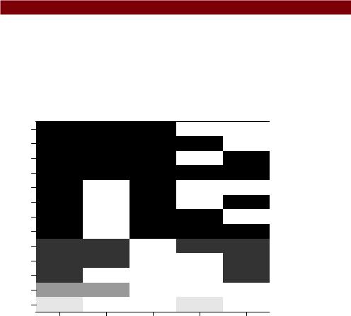
In listing 8.14, we’ll apply all subsets regression to the states data. The results can be plotted with either the plot() function in the leaps package or the subsets() function in the car package. An example of the former is provided infigure 8.17, and an example of the latter is given in figure 8.18.

Listing 8.14 All subsets regression

library(leaps)

leaps <-regsubsets(Murder ~ Population + Illiteracy + Income + Frost, data=states, nbest=4)

plot(leaps, scale="adjr2")

library(car)

subsets(leaps, statistic="cp",

main="Cp Plot for All Subsets Regression") abline(1,1,lty=2,col="red")

0.1

0.033

Figure 8.17 Best four models for each subset size based on Adjusted R-square

procedure can require significant computing time. In general, automated variable selection methods should be seen as an aid rather than a directing force in model selection. A well-fitting model that doesn’t make sense doesn’t help you. Ultimately, it’s your knowledge of the subject matter that should guide you.

8.7Taking the analysis further

We’ll end our discussion of regression by considering methods for assessing model generalizability and predictor relative importance.

8.7.1Cross-validation

In the previous section, we examined methods for selecting the variables to include in a regression equation. When description is your primary goal, the selection and interpretation of a regression model signals the end of your labor. But when your goal is prediction, you can justifiably ask, “How well will this equation perform in the real world?”

By definition, regression techniques obtain model parameters that are optimal for a given set of data. In OLS regression, the model parameters are selected to minimize the sum of squared errors of prediction (residuals), and conversely, maximize the amount of variance accounted for in the response variable (R-squared). Because the equation has been optimized for the given set of data, it won’t perform as well with a new set of data.

We began this chapter with an example involving a research physiologist who wanted to predict the number of calories an individual will burn from the duration and intensity of their exercise, age, gender, and BMI. If you fit an OLS regression equation to this data, you’ll obtain model parameters that uniquely maximize the R-squared for this particular set of observations. But our researcher wants to use this equation to predict the calories burned by individuals in general, not only those in the original study. You know that the equation won’t perform as well with a new sample of observations, but how much will you lose? Cross-validation is a useful method for evaluating the generalizability of a regression equation.

In cross-validation, a portion of the data is selected as the training sample and a portion is selected as the hold-out sample. A regression equation is developed on the training sample, and then applied to the hold-out sample. Because the hold-out sample wasn’t involved in the selection of the model parameters, the performance on this sample is a more accurate estimate of the operating characteristics of the model with new data.

In k-fold cross-validation, the sample is divided into k subsamples. Each of the k subsamples serves as a hold-out group and the combined observations from the remaining k-1 subsamples serves as the training group. The performance for the k prediction equations applied to the k hold-out samples are recorded and then averaged. (When k equals n, the total number of observations, this approach is called jackknifing.)

You can perform k-fold cross-validation using the crossval() function in the bootstrap package. The following listing provides a function (called shrinkage()) for cross-validating a model’s R-square statistic using k-fold cross-validation.

Listing 8.15 Function for k-fold cross-validated R-square

shrinkage <- function(fit, k=10){ require(bootstrap)

theta.fit <- function(x,y){lsfit(x,y)}

theta.predict <- function(fit,x){cbind(1,x)%*%fit$coef}

x <- fit$model[,2:ncol(fit$model)] y <- fit$model[,1]

results <- crossval(x, y, theta.fit, theta.predict, ngroup=k) r2 <- cor(y, fit$fitted.values)^2

r2cv <- cor(y, results$cv.fit)^2 cat("Original R-square =", r2, "\n")

cat(k, "Fold Cross-Validated R-square =", r2cv, "\n") cat("Change =", r2-r2cv, "\n")

}

Using this listing you define your functions, create a matrix of predictor and predicted values, get the raw R-squared, and get the cross-validated R-squared. ( Chapter 12 covers bootstrapping in detail.)

The shrinkage() function is then used to perform a 10-fold cross-validation with the states data, using a model with all four predictor variables:

>fit <- lm(Murder ~ Population + Income + Illiteracy + Frost, data=states)

>shrinkage(fit)

Original R-square=0.567

10 Fold Cross-Validated R-square=0.4481

Change=0.1188

You can see that the R-square based on our sample (0.567) is overly optimistic. A better estimate of the amount of variance in murder rates our model will account for with new data is the cross-validated R-square (0.448). (Note that observations are assigned to the k groups randomly, so you will get a slightly different result each time you execute the shrinkage() function.)

You could use cross-validation in variable selection by choosing a model that demonstrates better generalizability. For example, a model with two predictors (Population and Illiteracy) shows less R-square shrinkage (.03 versus .12) than the full model:

>fit2 <- lm(Murder~Population+Illiteracy,data=states)

>shrinkage(fit2)

Original R-square=0.5668327

10 Fold Cross-Validated R-square=0.5346871

Change=0.03214554

This may make the two-predictor model a more attractive alternative.

All other things being equal, a regression equation that’s based on a larger training sample and one that’s more representative of the population of interest will crossvalidate better. You’ll get less R-squared shrinkage and make more accurate predictions.

8.7.2Relative importance

Up to this point in the chapter, we’ve been asking, “Which variables are useful for predicting the outcome?” But often your real interest is in the question, “Which variables are most important in predicting the outcome?” You implicitly want to rank-order the predictors in terms of relative importance. There may be practical grounds for asking the second question. For example, if you could rank-order leadership practices by their relative importance for organizational success, you could help managers focus on the behaviors they most need to develop.

If predictor variables were uncorrelated, this would be a simple task. You would rank-order the predictor variables by their correlation with the response variable. In most cases, though, the predictors are correlated with each other, and this complicates the task significantly.

There have been many attempts to develop a means for assessing the relative importance of predictors. The simplest has been to compare standardized regression coefficients. Standardized regression coefficients describe the expected change in the response variable (expressed in standard deviation units) for a standard deviation change in a predictor variable, holding the other predictor variables constant. You can obtain the standardized regression coefficients in R by standardizing each of the variables in your dataset to a mean of 0 and standard deviation of 1 using the scale() function, before submitting the dataset to a regression analysis. (Note that because the scale() function returns a matrix and the lm() function requires a data frame, you convert between the two in an intermediate step.) The code and results for our multiple regression problem are shown here:

>zstates <- as.data.frame(scale(states))

>zfit <- lm(Murder~Population + Income + Illiteracy + Frost, data=zstates)

>coef(zfit)

Here you see that a one standard deviation increase in illiteracy rate yields a 0.68 standard deviation increase in murder rate, when controlling for population, income, and temperature. Using standardized regression coefficients as our guide, Illiteracy is the most important predictor and Frost is the least.

There have been many other attempts at quantifying relative importance. Relative importance can be thought of as the contribution each predictor makes to R-square, both alone and in combination with other predictors. Several possible approaches to relative importance are captured in the relaimpo package written by Ulrike Grömping (http://prof.beuth-hochschule.de/groemping/relaimpo/).