Robert I. Kabacoff - R in action

A new method called relative weights shows significant promise. The method closely approximates the average increase in R-square obtained by adding a predictor variable across all possible submodels (Johnson, 2004; Johnson and Lebreton, 2004; LeBreton and Tonidandel, 2008). A function for generating relative weights is provided in the next listing.

Listing 8.16 relweights() function for calculating relative importance of predictors

relweights <- function(fit,...){ R <- cor(fit$model)

nvar <- ncol(R)

rxx <- R[2:nvar, 2:nvar] rxy <- R[2:nvar, 1]

svd <- eigen(rxx) evec <- svd$vectors ev <- svd$values

delta <- diag(sqrt(ev))

lambda <- evec %*% delta %*% t(evec) lambdasq <- lambda ^ 2

beta <- solve(lambda) %*% rxy rsquare <- colSums(beta ^ 2) rawwgt <- lambdasq %*% beta ^ 2 import <- (rawwgt / rsquare) * 100 lbls <- names(fit$model[2:nvar]) rownames(import) <- lbls colnames(import) <- "Weights" barplot(t(import),names.arg=lbls,

ylab="% of R-Square", xlab="Predictor Variables",

main="Relative Importance of Predictor Variables", sub=paste("R-Square=", round(rsquare, digits=3)),

...) return(import)

}

NOTE The code in listing 8.16 is adapted from an SPSS program generously provided by Dr. Johnson. See Johnson (2000, Multivariate Behavioral Research, 35, 1–19) for an explanation of how the relative weights are derived.

In listing 8.17 the relweights() function is applied to the states data with murder rate predicted by the population, illiteracy, income, and temperature.

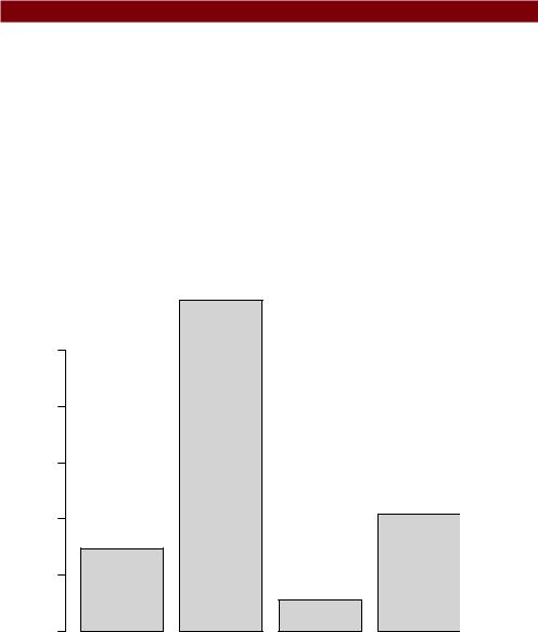
You can see from figure 8.19 that the total amount of variance accounted for by the model (R-square=0.567) has been divided among the predictor variables. Illiteracy accounts for 59 percent of the R-square, Frost accounts for 20.79 percent, and so forth. Based on the method of relative weights, Illiteracy has the greatest relative importance, followed by Frost, Population, and Income, in that order.

Listing 8.17 Applying the relweights() function

>fit <- lm(Murder ~ Population + Illiteracy + Income + Frost, data=states)

>relweights(fit, col="lightgrey")

Weights

Population 14.72

Illiteracy 59.00

Income 5.49

Frost 20.79

Relative importance measures (and in particular, the method of relative weights) have wide applicability. They come much closer to our intuitive conception of relative importance than standardized regression coefficients do, and I expect to see their use increase dramatically in coming years.

Relative Importance of Predictor Variables

% of R−Square 0 10 20 30 40 50

Predictor Variables

R−Square = 0.567

Figure 8.19 Bar plot of relative weights for the states multiple regression problem

8.8Summary

Regression analysis is a term that covers a broad range of methodologies in statistics. You’ve seen that it’s a highly interactive approach that involves fitting models, assessing their fit to statistical assumptions, modifying both the data and the models, and refitting to arrive at a final result. In many ways, this final result is based on art and skill as much as science.

This has been a long chapter, because regression analysis is a process with many parts. We’ve discussed fitting OLS regression models, using regression diagnostics to assess the data’s fit to statistical assumptions, and methods for modifying the data to meet these assumptions more closely. We looked at ways of selecting a final regression model from many possible models, and you learned how to evaluate its likely performance on new samples of data. Finally, we tackled the thorny problem of variable importance: identifying which variables are the most important for predicting an outcome.

In each of the examples in this chapter, the predictor variables have been quantitative. However, there are no restrictions against using categorical variables as predictors as well. Using categorical predictors such as gender, treatment type, or manufacturing process allows you to examine group differences on a response or outcome variable. This is the focus of our next chapter.

9.1A crash course on terminology

Experimental design in general, and analysis of variance in particular, has its own language. Before discussing the analysis of these designs, we’ll quickly review some important terms. We’ll use a series of increasingly complex study designs to introduce the most significant concepts.

Say you’re interested in studying the treatment of anxiety. Two popular therapies for anxiety are cognitive behavior therapy (CBT) and eye movement desensitization and reprocessing (EMDR). You recruit 10 anxious individuals and randomly assign half of them to receive five weeks of CBT and half to receive five weeks of EMDR. At the conclusion of therapy, each patient is asked to complete the State-Trait Anxiety

design is a one-way within-groups ANOVA. Because each subject is measured more than once, the design is also called repeated measures ANOVA. If the F test for Time is significant, you can conclude that patients’ mean STAI scores changed between five weeks and six months.

If you were interested in both treatment differences and change over time, you could combine the first two study designs, and randomly assign five patients to CBT and five patients to EMDR, and assess their STAI results at the end of therapy (five weeks) and at six months (see table 9.3).

By including both Therapy and Time as factors, you’re able to examine the impact of Therapy (averaged across time), Time (averaged across therapy type), and the interaction of Therapy and Time. The first two are called the main effects, whereas the interaction is (not surprisingly) called an interaction effect.

When you cross two or more factors, as you’ve done here, you have a factorial ANOVA design. Crossing two factors produces a two-way ANOVA, crossing three factors produces a three-way ANOVA, and so forth. When a factorial design includes both between-groups and within-groups factors, it’s also called a mixed-model ANOVA. The current design is a two-way mixed-model factorial ANOVA (phew!).

In this case you’ll have three F tests: one for Therapy, one for Time, and one for the Therapy x Time interaction. A significant result for Therapy indicates that CBT and EMDR differ in their impact on anxiety. A significant result for Time indicates that

Table 9.3 Two-way factorial ANOVA with one between-groups and one within-groups factor

anxiety changed from week five to the six month follow-up. A significant Therapy x Time interaction indicates that the two treatments for anxiety had a differential impact over time (that is, the change in anxiety from five weeks to six months was different for the two treatments).

Now let’s extend the design a bit. It’s known that depression can have an impact on therapy, and that depression and anxiety often co-occur. Even though subjects were randomly assigned to treatment conditions, it’s possible that the two therapy groups differed in patient depression levels at the initiation of the study. Any posttherapy differences might then be due to the preexisting depression differences and not to your experimental manipulation. Because depression could also explain the group differences on the dependent variable, it’s a confounding factor. And because you’re not interested in depression, it’s called a nuisance variable.

If you recorded depression levels using a self-report depression measure such as the Beck Depression Inventory (BDI) when patients were recruited, you could statistically adjust for any treatment group differences in depression before assessing the impact of therapy type. In this case, BDI would be called a covariate, and the design would be called an analysis of covariance (ANCOVA).

Finally, you’ve recorded a single dependent variable in this study (the STAI). You could increase the validity of this study by including additional measures of anxiety (such as family ratings, therapist ratings, and a measure assessing the impact of anxiety on their daily functioning). When there’s more than one dependent variable, the design is called a multivariate analysis of variance (MANOVA). If there are covariates present, it’s called a multivariate analysis of covariance (MANCOVA).

Now that you have the basic terminology under your belt, you’re ready to amaze your friends, dazzle new acquaintances, and discuss how to fit ANOVA/ANCOVA/ MANOVA models with R.

9.2Fitting ANOVA models

Although ANOVA and regression methodologies developed separately, functionally they’re both special cases of the general linear model. We could analyze ANOVA models using the same lm() function used for regression in chapter 7. However, we’ll primarily use the aov() function in this chapter. The results of lm() and aov() are equivalent, but the aov() function presents these results in a format that’s more familiar to ANOVA methodologists. For completeness, I’ll provide an example using lm()at the end of this chapter.

9.2.1The aov() function

The syntax of the aov() function is aov(formula, data=dataframe). Table 9.4 describes special symbols that can be used in the formulas. In this table, y is the dependent variable and the letters A, B, and C represent factors.

Table 9.4 Special symbols used in R formulas

~Separates response variables on the left from the explanator y variables on the right. For

example, a prediction of y from A, B, and C would be coded y ~ A + B + C.

+Separates explanator y variables.

:Denotes an interaction between variables. A prediction of y from A, B, and the

interaction between A and B would be coded y ~ A + B + A:B.

*Denotes the complete crossing variables. The code y ~ A*B*C expands to y ~ A + B + C + A:B + A:C + B:C + A:B:C.

^Denotes crossing to a specified degree. The code y ~ (A+B+C)^2 expands to y ~ A + B + C + A:B + A:C + A:B.

Table 9.5 provides formulas for several common research designs. In this table, lowercase letters are quantitative variables, uppercase letters are grouping factors, and Subject is a unique identifier variable for subjects.

Table 9.5 Formulas for common research designs

We’ll explore in-depth examples of several of these designs later in this chapter.

9.2.2The order of formula terms

The order in which the effects appear in a formula matters when (a) there’s more than one factor and the design is unbalanced, or (b) covariates are present. When either of these two conditions is present, the variables on the right side of the equation will be correlated with each other. In this case, there’s no unambiguous way to divide up their impact on the dependent variable.