

Robert I. Kabacoff - R in action
.pdf176 |
CHAPTER 8 Regression |
mathematical form of these relationships. She collects data on each of these variables from a representative sample of bridges and models the data using OLS regression.
The approach is highly interactive. She fits a series of models, checks their compliance with underlying statistical assumptions, explores any unexpected or aberrant findings, and finally chooses the “best” model from among many possible models. If successful, the results will help her to
Focus on important variables, by determining which of the many collected variables are useful in predicting bridge deterioration, along with their relative importance.
Look for bridges that are likely to be in trouble, by providing an equation that can be used to predict bridge deterioration for new cases (where the values of the predictor variables are known, but the degree of bridge deterioration isn’t). Take advantage of serendipity, by identifying unusual bridges. If she finds that some bridges deteriorate much faster or slower than predicted by the model, a study of these “outliers” may yield important findings that could help her to understand the mechanisms involved in bridge deterioration.
Bridges may hold no interest for you. I’m a clinical psychologist and statistician, and I know next to nothing about civil engineering. But the general principles apply to an amazingly wide selection of problems in the physical, biological, and social sciences. Each of the following questions could also be addressed using an OLS approach:
What’s the relationship between surface stream salinity and paved road surface area (Montgomery, 2007)?
What aspects of a user’s experience contribute to the overuse of massively multiplayer online role playing games (MMORPGs) (Hsu, Wen, & Wu, 2009)?
Which qualities of an educational environment are most strongly related to higher student achievement scores?
What’s the form of the relationship between blood pressure, salt intake, and age? Is it the same for men and women?
What’s the impact of stadiums and professional sports on metropolitan area development (Baade & Dye, 1990)?
What factors account for interstate differences in the price of beer (Culbertson & Bradford, 1991)? (That one got your attention!)
Our primary limitation is our ability to formulate an interesting question, devise a useful response variable to measure, and gather appropriate data.
8.1.2What you need to know
For the remainder of this chapter I’ll describe how to use R functions to fit OLS regression models, evaluate the fit, test assumptions, and select among competing models. It’s assumed that the reader has had exposure to least squares regression as typically taught in a second semester undergraduate statistics course. However, I’ve made

OLS regression |
177 |
efforts to keep the mathematical notation to a minimum and focus on practical rather than theoretical issues. A number of excellent texts are available that cover the statistical material outlined in this chapter. My favorites are John Fox’s Applied Regression Analysis and Generalized Linear Models (for theory) and An R and S-Plus Companion to Applied Regression (for application). They both served as major sources for this chapter. A good nontechnical overview is provided by Licht (1995).
8.2OLS regression
For most of this chapter, we’ll be predicting the response variable from a set of predictor variables (also called “regressing” the response variable on the predictor vari- ables—hence the name) using OLS. OLS regression fits models of the form
ˆ |
ˆ |
ˆ |
ˆ |
i = 1…n |
Yi |
= β0 |
+ β1 |
X1i + …+ βk Xki |
where n is the number of observations and k is the number of predictor variables. (Although I’ve tried to keep equations out of our discussions, this is one of the few places where it simplifies things.) In this equation:
n |
is the predicted value of the dependent variable for obser vation i (specifically, it’s the |
Y i |
estimated mean of the Y distribution, conditional on the set of predictor values) |
|
|
Xji |
is the jth predictor value for the ith obser vation |
nis the intercept (the predicted value of Y when all the predictor variables equal zero)
β0
nis the regression coefficient for the jth predictor (slope representing the change in Y for a unit
βj change in Xj)
Our goal is to select model parameters (intercept and slopes) that minimize the difference between actual response values and those predicted by the model. Specifically, model parameters are selected to minimize the sum of squared residuals
To properly interpret the coefficients of the OLS model, you must satisfy a number of statistical assumptions:
Normality —For fixed values of the independent variables, the dependent variable is normally distributed.
Independence —The Yi values are independent of each other.
Linearity —The dependent variable is linearly related to the independent variables.
Homoscedasticity —The variance of the dependent variable doesn’t vary with the levels of the independent variables. We could call this constant variance, but saying homoscedasticity makes me feel smarter.

178 |
CHAPTER 8 Regression |
If you violate these assumptions, your statistical significance tests and confidence intervals may not be accurate. Note that OLS regression also assumes that the independent variables are fixed and measured without error, but this assumption is typically relaxed in practice.
8.2.1Fitting regression models with lm()
In R, the basic function for fitting a linear model is lm(). The format is
myfit <- lm(formula, data)
where formula describes the model to be fit and data is the data frame containing the data to be used in fitting the model. The resulting object (myfit in this case) is a list that contains extensive information about the fitted model. The formula is typically written as
Y ~ X1 + X2 + … + Xk
where the ~ separates the response variable on the left from the predictor variables on the right, and the predictor variables are separated by + signs. Other symbols can be used to modify the formula in various ways (see table 8.2).
Table 8.2 Symbols commonly used in R formulas
Symbol |
Usage |
|
|
~ |
Separates response variables on the left from the explanator y variables on the right. |
|
For example, a prediction of y from x, z, and w would be coded y ~ x + z + w. |
+ |
Separates predictor variables. |
: |
Denotes an interaction between predictor variables. A prediction of y from x, z, and the |
|
interaction between x and z would be coded y ~ x + z + x:z. |
* |
A shor tcut for denoting all possible interactions. The code y ~ x * z * w expands |
|
to y ~ x + z + w + x:z + x:w + z:w + x:z:w. |
^ |
Denotes interactions up to a specified degree. The code y ~ (x + z + w)^2 |
|
expands to y ~ x + z + w + x:z + x:w + z:w. |
. |
A place holder for all other variables in the data frame except the dependent variable. |
|
For example, if a data frame contained the variables x, y, z, and w, then the code y |
|
~ . would expand to y ~ x + z + w. |
- |
A minus sign removes a variable from the equation. For example, y ~ (x + z + |
|
w)^2 – x:w expands to y ~ x + z + w + x:z + z:w. |
-1 |
Suppresses the intercept. For example, the formula y ~ x -1 fits a regression of y |
|
on x, and forces the line through the origin at x=0. |
I() |
Elements within the parentheses are interpreted arithmetically. For example, y ~ x + |
|
(z + w)^2 would expand to y ~ x + z + w + z:w. In contrast, the code y ~ x |
|
+ I((z + w)^2) would expand to y ~ x + h, where h is a new variable created by |
|
squaring the sum of z and w. |
function |
Mathematical functions can be used in formulas. For example, |
|
log(y) ~ x + z + w would predict log(y) from x, z, and w. |
|
|

OLS regression |
179 |
In addition to lm(), table 8.3 lists several functions that are useful when generating a simple or multiple regression analysis. Each of these functions is applied to the object returned by lm() in order to generate additional information based on that fitted model.
Function |
Action |
|
|
summary() |
Displays detailed results for the fitted model |
coefficients() |
Lists the model parameters (intercept and slopes) for the fitted model |
confint() |
Provides confidence inter vals for the model parameters (95 percent by |
|
default) |
fitted() |
Lists the predicted values in a fitted model |
residuals() |
Lists the residual values in a fitted model |
anova() |
Generates an ANOVA table for a fitted model, or an ANOVA table |
|
comparing two or more fitted models |
vcov() |
Lists the covariance matrix for model parameters |
AIC() |
Prints Akaike’s Information Criterion |
plot() |
Generates diagnostic plots for evaluating the fit of a model |
predict() |
Uses a fitted model to predict response values for a new dataset |
|
|
When the regression model contains one dependent variable and one independent variable, we call the approach simple linear regression. When there’s one predictor variable but powers of the variable are included (for example, X, X2, X3), we call it polynomial regression. When there’s more than one predictor variable, you call it multiple linear regression. We’ll start with an example of a simple linear regression, then progress to examples of polynomial and multiple linear regression, and end with an example of multiple regression that includes an interaction among the predictors.
8.2.2Simple linear regression
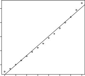
Let’s take a look at the functions in table 8.3 through a simple regression example. The dataset women in the base installation provides the height and weight for a set of 15 women ages 30 to 39. We want to predict weight from height. Having an equation for predicting weight from height can help us to identify overweight or underweight individuals. The analysis is provided in the following listing, and the resulting graph is shown in figure 8.1.
Listing 8.1 Simple linear regression
>fit <- lm(weight ~ height, data=women)
>summary(fit)
180 |
|
|
CHAPTER 8 |
Regression |
|
||
Call: |
|
|
|
|
|
|
|
lm(formula=weight ~ height, data=women) |
|
|
|||||
Residuals: |
|
|
|
|
|
|
|
Min |
1Q |
Median |
3Q |
Max |
|
|
|
-1.733 -1.133 |
-0.383 |
0.742 |
3.117 |
|
|
|
|
Coefficients: |
|
|
|
|
|
|
|
|
Estimate Std. Error t value Pr(>|t|) |
|
|||||
(Intercept) -87.5167 |
5.9369 |
-14.7 |
1.7e-09 |
*** |
|||
height |
|
3.4500 |
0.0911 |
37.9 |
1.1e-14 |
*** |
|
--- |
|
|
|
|
|
|
|
Signif. codes: |
0 '***' 0.001 '**' 0.01 |
'*' 0.05 |
'.' 0.1 '' 1 |
||||
Residual standard error: 1.53 on 13 degrees of freedom
Multiple R-squared: 0.991, Adjusted R-squared: 0.99
F-statistic: 1.43e+03 on 1 and 13 DF, p-value: 1.09e-14
>women$weight
[1]115 117 120 123 126 129 132 135 139 142 146 150 154 159 164
>fitted(fit)
1 |
2 |
|
3 |
|
4 |
|
5 |
|
6 |
7 |
|
8 |
|
9 |
112.58 |
116.03 |
119.48 |
122.93 |
126.38 |
|
129.83 |
133.28 |
136.73 |
140.18 |
|||||
10 |
11 |
|
12 |
|
13 |
|
14 |
|
15 |
|
|
|
|
|
143.63 |
147.08 |
150.53 |
153.98 |
157.43 |
|
160.88 |
|
|
|
|
|
|||
> residuals(fit) |
|
|
|
|
|
|
|
|
|
|
|
|
||
1 |
2 |
3 |
|
4 |
|
5 |
|
6 |
7 |
8 |
9 |
|
10 |
11 |
2.42 |
0.97 |
0.52 |
0.07 |
-0.38 |
-0.83 |
-1.28 |
-1.73 |
-1.18 |
-1.63 |
-1.08 |
||||
12 |
13 |
14 |
|
15 |
|
|
|
|
|
|
|
|
|
|
-0.53 |
0.02 |
1.57 |
3.12 |
|
|
|
|
|
|
|
|
|
|
|
>plot(women$height,women$weight, xlab="Height (in inches)", ylab="Weight (in pounds)")
>abline(fit)
From the output, you see that the prediction equation is
p
Weight = −87.52 + 3.45 × Height
Because a height of 0 is impossible, you wouldn’t try to give a physical interpretation to the intercept. It merely becomes an adjustment constant. From the Pr(>|t|) column, you see that the regression coefficient (3.45) is significantly different from zero (p < 0.001) and indicates that there’s an expected increase of 3.45 pounds of weight for every 1 inch increase in height. The multiple R-squared (0.991) indicates that the model accounts for 99.1 percent of the variance in weights. The multiple R-squared
is also the correlation between the actual and predicted value (that is, R2 = rYnY ). The residual standard error (1.53 lbs.) can be thought of as the average error in
OLS regression |
181 |
160 |
|
150 |
|
(in pounds) 140 |
|
Weight |
|
130 |
|
120 |
|
58 |
60 |
62 |
64 |
66 |
68 |
70 |
72 |
Figure 8.1 Scatter plot with |
|
regression line for weight |
|||||||||
|
|
|
|
|
|
|
|
||
|
|
|
Height (in inches) |
|
|
|
predicted from height |
||
predicting weight from height using this model. The F statistic tests whether the predictor variables taken together, predict the response variable above chance levels. Because there’s only one predictor variable in simple regression, in this example the F test is equivalent to the t-test for the regression coefficient for height.
For demonstration purposes, we’ve printed out the actual, predicted, and residual values. Evidently, the largest residuals occur for low and high heights, which can also be seen in the plot (figure 8.1).
The plot suggests that you might be able to improve on the prediction by using a |
||||
line with one bend. For example, a model of the form |
|
+ β1X + β2 X |
2 |
may provide |
Y = β0 |
|
|||
a better fit to the data. Polynomial regression allows you to predict a response variable from an explanatory variable, where the form of the relationship is an nth degree polynomial.
8.2.3Polynomial regression
The plot in figure 8.1 suggests that you might be able to improve your prediction using a regression with a quadratic term (that is, X 2).
You can fit a quadratic equation using the statement
fit2 <- lm(weight ~ height + I(height^2), data=women)
The new term I(height^2) requires explanation. height^2 adds a height-squared term to the prediction equation. The I function treats the contents within the parentheses as an R regular expression. You need this because the ^ operator has a special meaning in formulas that you don’t want to invoke here (see table 8.2).
Listing 8.2 shows the results of fitting the quadratic equation.

182 |
CHAPTER 8 Regression |
Listing 8.2 Polynomial regression
>fit2 <- lm(weight ~ height + I(height^2), data=women)
>summary(fit2)
Call:
lm(formula=weight ~ height + I(height^2), data=women)
Residuals: |
|
|
|
|
|
Min |
1Q |
Median |
3Q |
Max |
|
-0.5094 -0.2961 -0.0094 |
0.2862 |
0.5971 |
|
||
Coefficients: |
|
|
|
|
|
|
Estimate Std. Error t value Pr(>|t|) |
||||
(Intercept) 261.87818 |
25.19677 |
10.39 |
2.4e-07 *** |
||
height |
-7.34832 |
0.77769 |
-9.45 |
6.6e-07 *** |
|
I(height^2) |
0.08306 |
0.00598 |
13.89 |
9.3e-09 *** |
|
--- |
|
|
|
|
|
Signif. codes: |
0 '***' 0.001 '**' 0.01 '*' 0.05 '.' 0.1 ' ' 1 |
||||
Residual standard error: 0.384 on 12 degrees of freedom
Multiple R-squared: 0.999, Adjusted R-squared: 0.999
F-statistic: 1.14e+04 on 2 and 12 DF, p-value: <2e-16
>plot(women$height,women$weight, xlab="Height (in inches)", ylab="Weight (in lbs)")
>lines(women$height,fitted(fit2))
From this new analysis, the prediction equation is
and both regression coefficients are significant at the p < 0.0001 level. The amount of variance accounted for has increased to 99.9 percent. The significance of the squared term (t = 13.89, p < .001) suggests that inclusion of the quadratic term improves the model fit. If you look at the plot of fit2 (figure 8.2) you can see that the curve does indeed provides a better fit.
|
160 |
|
|
|
|
|
|
|
|
150 |
|
|
|
|
|
|
|
Weight (in lbs) |
140 |
|
|
|
|
|
|
|
|
130 |
|
|
|
|
|
|
|
|
120 |
|
|
|
|
|
|
|
|
58 |
60 |
62 |
64 |
66 |
68 |
70 |
72 |
Height (in inches)
Figure 8.2 Quadratic regression for weight predicted by height
OLS regression |
183 |
Linear versus nonlinear models
Note that this polynomial equation still fits under the rubric of linear regression. It’s linear because the equation involves a weighted sum of predictor variables (height and height-squared in this case). Even a model such as
would be considered a linear model (linear in terms of the parameters) and fit with the formula
Y ~ log(X1) + sin(X2)
In contrast, here’s an example of a truly nonlinear model:
Nonlinear models of this form can be fit with the nls() function.
In general, an nth degree polynomial produces a curve with n-1 bends. To fit a cubic polynomial, you’d use
fit3 <- lm(weight ~ height + I(height^2) +I(height^3), data=women)
Although higher polynomials are possible, I’ve rarely found that terms higher than cubic are necessary.
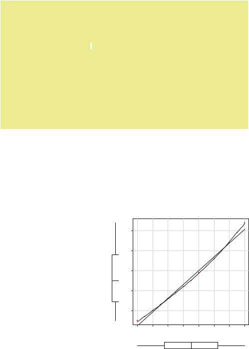
Before we move on, I should mention that the scatterplot() function in the car package provides a simple and convenient method of plotting a bivariate relationship. The code
library(car) scatterplot(weight ~ height,
data=women,
spread=FALSE, lty.smooth=2, pch=19,
main="Women Age 30-39", xlab="Height (inches)", ylab="Weight (lbs.)")
produces the graph in figure 8.3. This enhanced plot provides the
scatter plot of weight with height, box plots for each variable in their respective margins, the linear line of best fit, and a smoothed (loess) fit line. The spread=FALSE options suppress spread and asymmetry information. The lty.smooth=2 option specifies that the loess fit be rendered as a dashed line. The
|
160 |
|
|
|
|
|
|
|
|
150 |
|
|
|
|
|
|
|
Weight (lbs.) |
140 |
|
|
|
|
|
|
|
|
130 |
|
|
|
|
|
|
|
|
120 |
|
|
|
|
|
|
|
|
58 |
60 |
62 |
64 |
66 |
68 |
70 |
72 |
|
|
|
|
Height (inches) |
|
|
|
|
Figure 8.3 Scatter plot of height by weight, with linear and smoothed fits, and marginal box plots

184 |
CHAPTER 8 Regression |
pch=19 options display points as filled circles (the default is open circles). You can tell at a glance that the two variables are roughly symmetrical and that a curved line will fit the data points better than a straight line.
8.2.4Multiple linear regression
When there’s more than one predictor variable, simple linear regression becomes multiple linear regression, and the analysis grows more involved. Technically, polynomial regression is a special case of multiple regression. Quadratic regression has two predictors (X and X 2), and cubic regression has three predictors (X, X 2, and X 3). Let’s look at a more general example.
We’ll use the state.x77 dataset in the base package for this example. We want to explore the relationship between a state’s murder rate and other characteristics of the state, including population, illiteracy rate, average income, and frost levels (mean number of days below freezing).
Because the lm() function requires a data frame (and the state.x77 dataset is contained in a matrix), you can simplify your life with the following code:
states <- as.data.frame(state.x77[,c("Murder", "Population", "Illiteracy", "Income", "Frost")])
This code creates a data frame called states, containing the variables we’re interested in. We’ll use this new data frame for the remainder of the chapter.
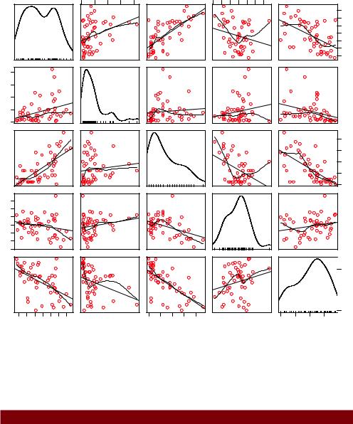
A good first step in multiple regression is to examine the relationships among the variables two at a time. The bivariate correlations are provided by the cor() function, and scatter plots are generated from the scatterplotMatrix() function in the car package (see the following listing and figure 8.4).
Listing 8.3 Examining bivariate relationships
> cor(states) |
|
|
|
|
|
|
Murder Population Illiteracy Income Frost |
||||
Murder |
1.00 |
0.34 |
0.70 |
-0.23 -0.54 |
|
Population |
0.34 |
1.00 |
0.11 |
0.21 |
-0.33 |
Illiteracy |
0.70 |
0.11 |
1.00 |
-0.44 |
-0.67 |
Income |
-0.23 |
0.21 |
-0.44 |
1.00 |
0.23 |
Frost |
-0.54 |
-0.33 |
-0.67 |
0.23 |
1.00 |
>library(car)
>scatterplotMatrix(states, spread=FALSE, lty.smooth=2, main="Scatter Plot Matrix")
By default, the scatterplotMatrix() function provides scatter plots of the variables with each other in the off-diagonals and superimposes smoothed (loess) and linear fit lines on these plots. The principal diagonal contains density and rug plots for each variable.
You can see that murder rate may be bimodal and that each of the predictor variables is skewed to some extent. Murder rates rise with population and illiteracy, and fall with higher income levels and frost. At the same time, colder states have lower illiteracy rates and population and higher incomes.
OLS regression |
185 |
Murder |
20000 |
10000 |
0 |
6000 |
4500 |
3000 |
2 |
6 |
10 |
14 |
Scatterplot Matrix
0 |
10000 |
20000 |
Population |
||
3000 |
4500 |
6000 |
Illiteracy |
Income
0.5 |
1.5 |
2.5 |
14 |
10 |
6 |
2 |
2.5 |
1.5 |
0.5 |
Frost
 0 50 100
0 50 100
Figure 8.4 Scatter plot matrix of dependent and independent variables for the states data, including linear and smoothed fits, and marginal distributions (kernel density plots and rug plots)
Now let’s fit the multiple regression model with the lm() function (see the following listing).
Listing 8.4 Multiple linear regression
> fit <- lm(Murder ~ Population + Illiteracy + Income + Frost, data=states)
> summary(fit)
Call:
lm(formula=Murder ~ Population + Illiteracy + Income + Frost, data=states)