Robert I. Kabacoff - R in action

1x equals c(1, 2, 3, 4, 5, 6, 7, 8) and mean x equals 4.5 (length(x) returns the number of elements in x).

2(x – meanx) subtracts 4.5 from each element of x, resulting in c(-3.5, -2.5, -1.5, -0.5, 0.5, 1.5, 2.5, 3.5).

3(x – meanx)^2 squares each element of (x - meanx), resulting in c(12.25, 6.25, 2.25, 0.25, 0.25, 2.25, 6.25, 12.25).

4sum((x - meanx)^2) sums each of the elements of (x - meanx)^2), resulting in 42.

Writing formulas in R has much in common with matrix manipulation languages such as MATLAB (we’ll look more specifically at solving matrix algebra problems in appendix E).

STANDARDIZING DATA

By default, the scale() function standardizes the specified columns of a matrix or data frame to a mean of 0 and a standard deviation of 1:

newdata <- scale(mydata)

To standardize each column to an arbitrary mean and standard deviation, you can use code similar to the following:

newdata <- scale(mydata)*SD + M

where M is the desired mean and SD is the desired standard deviation. Using the scale() function on non-numeric columns will produce an error. To standardize a specific column rather than an entire matrix or data frame, you can use code such as

newdata <- transform(mydata, myvar = scale(myvar)*10+50)

This code standardizes the variable myvar to a mean of 50 and standard deviation of 10. We’ll use the scale() function in the solution to the data management challenge in section 5.3.

5.2.3Probability functions

You may wonder why probability functions aren’t listed with the statistical functions (it was really bothering you, wasn’t it?). Although probability functions are statistical by definition, they’re unique enough to deserve their own section. Probability functions are often used to generate simulated data with known characteristics and to calculate probability values within user-written statistical functions.

In R, probability functions take the form

[dpqr]distribution_abbreviation()

where the first letter refers to the aspect of the distribution returned: d = density

p= distribution function

q= quantile function

r= random generation (random deviates)

The common probability functions are listed in table 5.4.

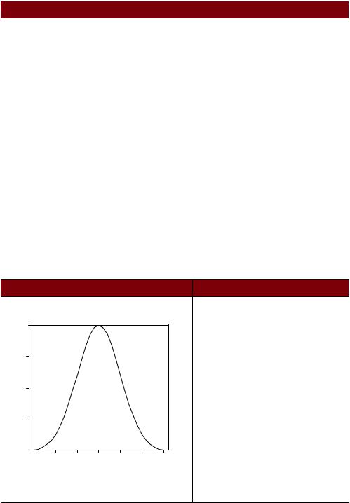
To see how these work, let’s look at functions related to the normal distribution. If you don’t specify a mean and a standard deviation, the standard normal distribution is assumed (mean=0, sd=1). Examples of the density (dnorm), distribution (pnorm), quantile (qnorm) and random deviate generation (rnorm) functions are given in table 5.5.

Table 5.5 Normal distribution functions

Normal Deviate

Don’t worry if the plot function options are unfamiliar. They’re covered in detail in chapter 11; pretty() is explained in table 5.7 later in this chapter.

SETTING THE SEED FOR RANDOM NUMBER GENERATION

Each time you generate pseudo-random deviates, a different seed, and therefore different results, are produced. To make your results reproducible, you can specify the seed explicitly, using the set.seed() function. An example is given in the next listing. Here, the runif() function is used to generate pseudo-random numbers from a uniform distribution on the interval 0 to 1.

Listing 5.2 Generating pseudo-random numbers from a uniform distribution

> runif(5)

[1] 0.8725344 0.3962501 0.6826534 0.3667821 0.9255909 > runif(5)

[1] 0.4273903 0.2641101 0.3550058 0.3233044 0.6584988

>set.seed(1234)

>runif(5)

[1] 0.1137034 0.6222994 0.6092747 0.6233794 0.8609154

>set.seed(1234)

>runif(5)

[1] 0.1137034 0.6222994 0.6092747 0.6233794 0.8609154

By setting the seed manually, you’re able to reproduce your results. This ability can be helpful in creating examples you can access at a future time and share with others.

GENERATING MULTIVARIATE NORMAL DATA

In simulation research and Monte Carlo studies, you often want to draw data from multivariate normal distribution with a given mean vector and covariance matrix. The mvrnorm() function in the MASS package makes this easy. The function call is

mvrnorm(n, mean, sigma)

where n is the desired sample size, mean is the vector of means, and sigma is the vari- ance-covariance (or correlation) matrix. In listing 5.3 you’ll sample 500 observations from a three-variable multivariate normal distribution with

Listing 5.3 Generating data from a multivariate normal distribution

>library(MASS)

>options(digits=3)

> set.seed(1234) .Set random number seed

>mydata <- as.data.frame(mydata)

>names(mydata) <- c("y","x1","x2")

198.8 41.3 4.35

2244.5 205.2 3.57

3375.7 186.7 3.69

4-59.2 11.2 4.23

5313.0 111.0 2.91

6288.8 185.1 4.18

7134.8 165.0 3.68

8171.7 97.4 3.81

9167.3 101.0 4.01

10121.1 94.5 3.76

In listing 5.3, you set a random number seed so that you can reproduce the results at a later time .. You specify the desired mean vector and variance-covariance matrix 3, and generate 500 pseudo-random observations $. For convenience, the results are converted from a matrix to a data frame, and the variables are given names. Finally, you confirm that you have 500 observations and 3 variables, and print out the first 10 observations /. Note that because a correlation matrix is also a covariance matrix, you could’ve specified the correlations structure directly.

The probability functions in R allow you to generate simulated data, sampled from distributions with known characteristics. Statistical methods that rely on simulated data have grown exponentially in recent years, and you’ll see several examples of these in later chapters.

5.2.4Character functions

Although mathematical and statistical functions operate on numerical data, character functions extract information from textual data, or reformat textual data for printing and reporting. For example, you may want to concatenate a person’s first name and last name, ensuring that the first letter of each is capitalized. Or you may want to count the instances of obscenities in open-ended feedback. Some of the most useful character functions are listed in table 5.6.

Note that the functions grep(), sub(), and strsplit() can search for a text string (fixed=TRUE) or a regular expression (fixed=FALSE) (FALSE is the default). Regular expressions provide a clear and concise syntax for matching a pattern of text. For example, the regular expression

^[hc]?at

matches any string that starts with 0 or one occurrences of h or c, followed by at. The expression therefore matches hat, cat, and at, but not bat. To learn more, see the regular expression entry in Wikipedia.

5.2.5Other useful functions

The functions in table 5.7 are also quite useful for data management and manipulation, but they don’t fit cleanly into the other categories.

Table 5.7 Other useful functions

The last example in the table demonstrates the use of escape characters in printing. Use \n for new lines, \t for tabs, \' for a single quote, \b for backspace, and so forth (type ?Quotes for more information). For example, the code

name <- "Bob"

cat( "Hello", name, "\b.\n", "Isn\'t R", "\t", "GREAT?\n")

102 CHAPTER 5 Advanced data management

produces

Note that the second line is indented one space. When cat concatenates objects for output, it separates each by a space. That’s why you include the backspace (\b) escape character before the period. Otherwise it would have produced “Hello Bob .”

How you apply the functions you’ve covered so far to numbers, strings, and vectors is intuitive and straightforward, but how do you apply them to matrices and data frames? That’s the subject of the next section.

5.2.6Applying functions to matrices and data frames

One of the interesting features of R functions is that they can be applied to a variety of data objects (scalars, vectors, matrices, arrays, and data frames). The following listing provides an example.

Listing 5.4 Applying functions to data objects

>a <- 5

>sqrt(a) [1] 2.236068

>b <- c(1.243, 5.654, 2.99)

>round(b)

[1] 1 6 3

>c <- matrix(runif(12), nrow=3)

>c

Notice that the mean of matrix c in listing 5.4 results in a scalar (0.444). The mean() function took the average of all 12 elements in the matrix. But what if you wanted the 3 row means or the 4 column means?

R provides a function, apply(), that allows you to apply an arbitrary function to any dimension of a matrix, array, or data frame. The format for the apply function is

apply(x, MARGIN, FUN, ...)

where x is the data object, MARGIN is the dimension index, FUN is a function you specify, and ... are any parameters you want to pass to FUN. In a matrix or data frame MARGIN=1 indicates rows and MARGIN=2 indicates columns. Take a look at the examples in listing 5.5.

[10,] 0.243 -0.077 -0.697

Step 3. You can then get a performance score for each student by calculating the row means using the mean() function and adding it to the roster using the cbind() function:

>score <- apply(z, 1, mean)

>roster <- cbind(roster, score)

>roster

Step 4. The quantile() function gives you the percentile rank of each student’s performance score. You see that the cutoff for an A is 0.74, for a B is 0.44, and so on.

>y <- quantile(roster$score, c(.8,.6,.4,.2))

>y

80% 60% 40% 20%

0.740.44 -0.36 -0.89

Step 5. Using logical operators, you can recode students’ percentile ranks into a new categorical grade variable. This creates the variable grade in the roster data frame.

>roster$grade[score >= y[1]] <- "A"

>roster$grade[score < y[1] & score >= y[2]] <- "B"

>roster$grade[score < y[2] & score >= y[3]] <- "C"

>roster$grade[score < y[3] & score >= y[4]] <- "D"

>roster$grade[score < y[4]] <- "F"

>roster