Robert I. Kabacoff - R in action

■There are some interesting exceptions. Railroad Engineers have high income and low education. Ministers have high prestige and low income.

■Education and (to lesser extent) prestige are distributed bi-modally, with more scores in the high and low ends than in the middle.

Chapter 8 will have much more to say about this type of graph. The important point is that R allows you to create elegant, informative, and highly customized graphs in a simple and straightforward fashion. Creating similar plots in other statistical languages would be difficult, time consuming, or impossible.

Unfortunately, R can have a steep learning curve. Because it can do so much, the documentation and help files available are voluminous. Additionally, because much of the functionality comes from optional modules created by independent contributors, this documentation can be scattered and difficult to locate. In fact, getting a handle on all that R can do is a challenge.

The goal of this book is to make access to R quick and easy. We’ll tour the many features of R, covering enough material to get you started on your data, with pointers on where to go when you need to learn more. Let’s begin by installing the program.

1.2Obtaining and installing R

R is freely available from the Comprehensive R Archive Network (CRAN) at http:// cran.r-project.org. Precompiled binaries are available for Linux, Mac OS X, and Windows. Follow the directions for installing the base product on the platform of your choice. Later we’ll talk about adding functionality through optional modules called packages (also available from CRAN). Appendix H describes how to update an existing R installation to a newer version.

1.3Working with R

R is a case-sensitive, interpreted language. You can enter commands one at a time at the command prompt (>) or run a set of commands from a source file. There are a wide variety of data types, including vectors, matrices, data frames (similar to datasets), and lists (collections of objects). We’ll discuss each of these data types in chapter 2.

Most functionality is provided through built-in and user-created functions, and all data objects are kept in memory during an interactive session. Basic functions are available by default. Other functions are contained in packages that can be attached to a current session as needed.

Statements consist of functions and assignments. R uses the symbol <- for assignments, rather than the typical = sign. For example, the statement

x <- rnorm(5)

creates a vector object named x containing five random deviates from a standard normal distribution.

NOTE R allows the = sign to be used for object assignments. However, you won’t find many programs written that way, because it’s not standard syntax, there are some situations in which it won’t work, and R programmers will make fun of you. You can also reverse the assignment direction. For instance, rnorm(5) -> x is equivalent to the previous statement. Again, doing so is uncommon and isn’t recommended in this book.

Comments are preceded by the # symbol. Any text appearing after the # is ignored by the R interpreter.

1.3.1Getting started

If you’re using Windows, launch R from the Start Menu. On a Mac, double-click the R icon in the Applications folder. For Linux, type R at the command prompt of a terminal window. Any of these will start the R interface(see figure 1.3 for an example).

To get a feel for the interface, let’s work through a simple contrived example. Say that you’re studying physical development and you’ve collected the ages and weights of 10 infants in their first year of life (see table 1.1). You’re interested in the distribution of the weights and their relationship to age.

Figure 1.3 Example of the R interface on Windows

Note: These are fictional data.

You’ll enter the age and weight data as vectors, using the function c(), which combines its arguments into a vector or list. Then you’ll get the mean and standard deviation of the weights, along with the correlation between age and weight, and plot the relationship between age and weight so that you can inspect any trend visually. The q() function, as shown in the following listing, will end the session and allow you to quit.

Listing 1.1 A sample R session

>age <- c(1,3,5,2,11,9,3,9,12,3)

>weight <- c(4.4,5.3,7.2,5.2,8.5,7.3,6.0,10.4,10.2,6.1)

>mean(weight)

[1] 7.06

>sd(weight) [1] 2.077498

>cor(age,weight) [1] 0.9075655

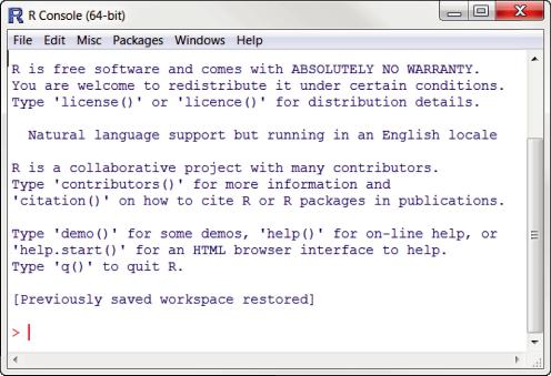
>plot(age,weight)

>q()

You can see from listing 1.1 that the mean weight for these 10 infants is 7.06 kilograms, that the standard deviation is 2.08 kilograms, and that there is strong linear relationship between age in months and weight in kilograms (correlation = 0.91). The relationship can also be seen in the scatter plot in figure 1.4. Not surprisingly, as infants get older, they tend to weigh more.

The scatter plot in figure 1.4 is informative but somewhat utilitarian and unattractive. In later chapters, you’ll see how to customize graphs to suit your needs.

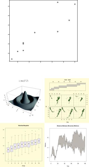
TIP To get a sense of what R can do graphically, enter demo(graphics)at the command prompt. A sample of the graphs produced is included in figure 1.5. Other demonstrations include demo(Hershey), demo(persp), and demo(image). To see a complete list of demonstrations, enter demo() without parameters.

1.3.2Getting help

R provides extensive help facilities, and learning to navigate them will help you significantly in your programming efforts. The built-in help system provides details, references, and examples of any function contained in a currently installed package. Help is obtained using the functions listed in table 1.2.

Table 1.2 R help functions

The function help.start() opens a browser window with access to introductory and advanced manuals, FAQs, and reference materials. The RSiteSearch() function searches for a given topic in online help manuals and archives of the R-Help discussion list and returns the results in a browser window. The vignettes returned by the vignette() function are practical introductory articles provided in PDF format. Not all packages will have vignettes. As you can see, R provides extensive help facilities, and learning to navigate them will definitely aid your programming efforts. It’s a rare session that I don’t use the ? to look up the features (such as options or return values) of some function.

1.3.3The workspace

The workspace is your current R working environment and includes any user-defined objects (vectors, matrices, functions, data frames, or lists). At the end of an R session, you can save an image of the current workspace that’s automatically reloaded the next time R starts. Commands are entered interactively at the R user prompt. You can use the

up and down arrow keys to scroll through your command history. Doing so allows you to select a previous command, edit it if desired, and resubmit it using the Enter key.

The current working directory is the directory R will read files from and save results to by default. You can find out what the current working directory is by using the getwd() function. You can set the current working directory by using the setwd() function. If you need to input a file that isn’t in the current working directory, use the full pathname in the call. Always enclose the names of files and directories from the operating system in quote marks.

Some standard commands for managing your workspace are listed in table 1.3.

Table 1.3 Functions for managing the R workspace

To see these commands in action, take a look at the following listing.

Listing 1.2 An example of commands used to manage the R workspace

setwd("C:/myprojects/project1")

options()

options(digits=3) x <- runif(20) summary(x) hist(x) savehistory() save.image()

q()

First, the current working directory is set to C:/myprojects/project1, the current option settings are displayed, and numbers are formatted to print with three digits after the decimal place. Next, a vector with 20 uniform random variates is created, and summary statistics and a histogram based on this data are generated. Finally, the command history is saved to the file .Rhistory, the workspace (including vector x) is saved to the file .RData, and the session is ended.

Note the forward slashes in the pathname of the setwd() command. R treats the backslash (\) as an escape character. Even when using R on a Windows platform, use forward slashes in pathnames. Also note that the setwd() function won’t create a directory that doesn’t exist. If necessary, you can use the dir.create() function to create a directory, and then use setwd() to change to its location.

It’s a good idea to keep your projects in separate directories. I typically start an R session by issuing the setwd() command with the appropriate path to a project, followed by the load() command without options. This lets me start up where I left off in my last session and keeps the data and settings separate between projects. On Windows and Mac OS X platforms, it’s even easier. Just navigate to the project directory and double-click on the saved image file. Doing so will start R, load the saved workspace, and set the current working directory to this location.

1.3.4Input and output

By default, launching R starts an interactive session with input from the keyboard and output to the screen. But you can also process commands from a script file (a file containing R statements) and direct output to a variety of destinations.

INPUT

The source("filename") function submits a script to the current session. If the filename doesn’t include a path, the file is assumed to be in the current working directory. For example, source("myscript.R") runs a set of R statements contained in file myscript.R. By convention, script file names end with an .R extension, but this isn’t required.

TEXT OUTPUT

The sink("filename") function redirects output to the file filename. By default, if the file already exists, its contents are overwritten. Include the option append=TRUE to append text to the file rather than overwriting it. Including the option split=TRUE will send output to both the screen and the output file. Issuing the command sink() without options will return output to the screen alone.

GRAPHIC OUTPUT

Although sink()redirects text output, it has no effect on graphic output. To redirect graphic output, use one of the functions listed in table 1.4. Use dev.off() to return output to the terminal.

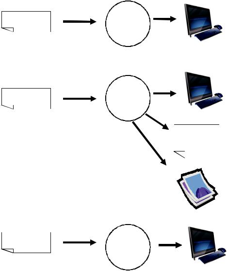
Let’s put it all together with an example. Assume that you have three script files containing R code (script1.R, script2.R, and script3.R). Issuing the statement

source("script1.R")

will submit the R code from script1.R to the current session and the results will appear on the screen.

If you then issue the statements

sink("myoutput", append=TRUE, split=TRUE) pdf("mygraphs.pdf")

source("script2.R")

the R code from file script2.R will be submitted, and the results will again appear on the screen. In addition, the text output will be appended to the file myoutput, and the graphic output will be saved to the file mygraphs.pdf.

Finally, if you issue the statements

sink()

dev.off()

source("script3.R")

the R code from script3.R will be submitted, and the results will appear on the screen. This time, no text or graphic output is saved to files. The sequence is outlined in figure 1.6.

R provides quite a bit of flexibility and control over where input comes from and where it goes. In section 1.5 you’ll learn how to run a program in batch mode.

1.4Packages

R comes with extensive capabilities right out of the box. But some of its most exciting features are available as optional modules that you can download and install. There are over 2,500 user-contributed modules called packages that you can download from http://cran.r-project.org/web/packages. They provide a tremendous range of new capabilities, from the analysis of geostatistical data to protein mass spectra processing to the analysis of psychological tests! You’ll use many of these optional packages in this book.

sink("myoutput", append=TRUE, split=TRUE)

myoutput

Output added

to the file

pdf("mygraphs.pdf")

sink(), dev.o ()

source("script3.R")

Figure 1.6 Input with the source() function and output with the sink() function

1.4.1What are packages?

Packages are collections of R functions, data, and compiled code in a well-defined format. The directory where packages are stored on your computer is called the library. The function .libPaths() shows you where your library is located, and the function library() shows you what packages you’ve saved in your library.