

Robert I. Kabacoff - R in action
.pdf106 |
CHAPTER 5 Advanced data management |
|
||||
9 |
Joel England |
573 |
89 |
27 |
0.698 |
B |
10 |
Mary Rayburn |
522 |
86 |
18 |
-0.177 |
C |
Step 6. You’ll use the strsplit() function to break student names into first name and last name at the space character. Applying strsplit() to a vector of strings returns a list:
>name <- strsplit((roster$Student), " ")
>name
[[1]]
[1] "John" "Davis"
[[2]]
[1] "Angela" "Williams"
[[3]]
[1] "Bullwinkle" "Moose"
[[4]]
[1] "David" "Jones"
[[5]]
[1] "Janice" "Markhammer"
[[6]]
[1] "Cheryl" "Cushing"
[[7]]
[1] "Reuven" "Ytzrhak"
[[8]]
[1] "Greg" "Knox"
[[9]]
[1] "Joel" "England"
[[10]]
[1] "Mary" "Rayburn"
Step 7. You can use the sapply() function to take the first element of each component and put it in a firstname vector, and the second element of each component and put it in a lastname vector. "[" is a function that extracts part of an object—here the first or second component of the list name. You’ll use cbind() to add them to the roster. Because you no longer need the student variable, you’ll drop it (with the –1 in the roster index).
>Firstname <- sapply(name, "[", 1)
>Lastname <- sapply(name, "[", 2)
>roster <- cbind(Firstname, Lastname, roster[,-1])
>roster
|
Firstname |
Lastname Math Science English |
score grade |
||||
1 |
John |
Davis |
502 |
95 |
25 |
0.559 |
B |
2 |
Angela |
Williams |
600 |
99 |
22 |
0.924 |
A |
3 |
Bullwinkle |
Moose |
412 |
80 |
18 |
-0.857 |
D |
|
|
|
|
Control flow |
|
|
107 |
4 |
David |
Jones |
358 |
82 |
15 |
-1.162 |
F |
5 |
Janice Markhammer |
495 |
75 |
20 |
-0.629 |
D |
|
6 |
Cheryl |
Cushing |
512 |
85 |
28 |
0.353 |
C |
7 |
Reuven |
Ytzrhak |
410 |
80 |
15 |
-1.048 |
F |
8 |
Greg |
Knox |
625 |
95 |
30 |
1.338 |
A |
9 |
Joel |
England |
573 |
89 |
27 |
0.698 |
B |
10 |
Mary |
Rayburn |
522 |
86 |
18 |
-0.177 |
C |
Step 8. Finally, you can sort the dataset by first and last name using the order() function:
> roster[order(Lastname,Firstname),] |
|
|
|
||||
|
Firstname |
Lastname |
Math |
Science |
English |
score |
grade |
6 |
Cheryl |
Cushing |
512 |
85 |
28 |
0.35 |
C |
1 |
John |
Davis |
502 |
95 |
25 |
0.56 |
B |
9 |
Joel |
England |
573 |
89 |
27 |
0.70 |
B |
4 |
David |
Jones |
358 |
82 |
15 |
-1.16 |
F |
8 |
Greg |
Knox |
625 |
95 |
30 |
1.34 |
A |
5 |
Janice Markhammer |
495 |
75 |
20 |
-0.63 |
D |
|
3 |
Bullwinkle |
Moose |
412 |
80 |
18 |
-0.86 |
D |
10 |
Mary |
Rayburn |
522 |
86 |
18 |
-0.18 |
C |
2 |
Angela |
Williams |
600 |
99 |
22 |
0.92 |
A |
7 |
Reuven |
Ytzrhak |
410 |
80 |
15 |
-1.05 |
F |
Voilà! Piece of cake!
There are many other ways to accomplish these tasks, but this code helps capture the flavor of these functions. Now it’s time to look at control structures and user-written functions.
5.4Control flow
In the normal course of events, the statements in an R program are executed sequentially from the top of the program to the bottom. But there are times that you’ll want to execute some statements repetitively, while only executing other statements if certain conditions are met. This is where control-flow constructs come in.
R has the standard control structures you’d expect to see in a modern programming language. First you’ll go through the constructs used for conditional execution, followed by the constructs used for looping.
For the syntax examples throughout this section, keep the following in mind:
■statement is a single R statement or a compound statement (a group of R statements enclosed in curly braces { } and separated by semicolons).
■cond is an expression that resolves to true or false.
■expr is a statement that evaluates to a number or character string.
■seq is a sequence of numbers or character strings.
After we discuss control-flow constructs, you’ll learn how to write your functions.
5.4.1Repetition and looping
Looping constructs repetitively execute a statement or series of statements until a condition isn’t true. These include the for and while structures.
108 |
CHAPTER 5 Advanced data management |
FOR
The for loop executes a statement repetitively until a variable’s value is no longer contained in the sequence seq. The syntax is
for (var in seq) statement
In this example
for (i in 1:10) print("Hello")
the word Hello is printed 10 times.
WHILE
A while loop executes a statement repetitively until the condition is no longer true. The syntax is
while (cond) statement
In a second example, the code
i <- 10
while (i > 0) {print("Hello"); i <- i - 1}
once again prints the word Hello 10 times. Make sure that the statements inside the brackets modify the while condition so that sooner or later it’s no longer true—other- wise the loop will never end! In the previous example, the statement
i <- i - 1
subtracts 1 from object i on each loop, so that after the tenth loop it’s no longer larger than 0. If you instead added 1 on each loop, R would never stop saying Hello. This is why while loops can be more dangerous than other looping constructs.
Looping in R can be inefficient and time consuming when you’re processing the rows or columns of large datasets. Whenever possible, it’s better to use R’s builtin numerical and character functions in conjunction with the apply family of functions.
5.4.2Conditional execution
In conditional execution, a statement or statements are only executed if a specified condition is met. These constructs include if-else, ifelse, and switch.
IF-ELSE
The if-else control structure executes a statement if a given condition is true. Optionally, a different statement is executed if the condition is false. The syntax is
if (cond) statement
if (cond) statement1 else statement2
Here are examples:
if (is.character(grade)) grade <- as.factor(grade)
if (!is.factor(grade)) grade <- as.factor(grade) else print("Grade already is a factor")

User-written functions |
109 |
In the first instance, if grade is a character vector, it’s converted into a factor. In the second instance, one of two statements is executed. If grade isn’t a factor (note the ! symbol), it’s turned into one. If it is a factor, then the message is printed.
IFELSE
The ifelse construct is a compact and vectorized version of the if-else construct. The syntax is
ifelse(cond, statement1, statement2)
The first statement is executed if cond is TRUE. If cond is FALSE, the second statement is executed. Here are examples:
ifelse(score > 0.5, print("Passed"), print("Failed")) outcome <- ifelse (score > 0.5, "Passed", "Failed")
Use ifelse when you want to take a binary action or when you want to input and output vectors from the construct.
SWITCH
switch chooses statements based on the value of an expression. The syntax is
switch(expr, ...)
where ... represents statements tied to the possible outcome values of expr. It’s easiest to understand how switch works by looking at the example in the following listing.
Listing 5.7 A switch example
>feelings <- c("sad", "afraid")
>for (i in feelings)
print( |
|
switch(i, |
|
happy |
= "I am glad you are happy", |
afraid |
= "There is nothing to fear", |
sad |
= "Cheer up", |
angry |
= "Calm down now" |
) |
|
) |
|
[1] "Cheer up" |
|
[1] "There is nothing to fear" |
|
This is a silly example but shows the main features. You’ll learn how to use switch in |
|
user-written functions in the next section. |
|
5.5 User-written functions
One of R’s greatest strengths is the user’s ability to add functions. In fact, many of the functions in R are functions of existing functions. The structure of a function looks like this:
myfunction <- function(arg1, arg2, ... ){ statements
return(object)
}

110 |
CHAPTER 5 Advanced data management |
Objects in the function are local to the function. The object returned can be any data type, from scalar to list. Let’s take a look at an example.
Say you’d like to have a function that calculates the central tendency and spread of data objects. The function should give you a choice between parametric (mean and standard deviation) and nonparametric (median and median absolute deviation) statistics. The results should be returned as a named list. Additionally, the user should have the choice of automatically printing the results, or not. Unless otherwise specified, the function’s default behavior should be to calculate parametric statistics and not print the results. One solution is given in the following listing.
Listing 5.8 mystats(): a user-written function for summary statistics
mystats <- function(x, parametric=TRUE, print=FALSE) { if (parametric) {
center <- mean(x); spread <- sd(x)
}else {
center <- median(x); spread <- mad(x)
}
if (print & parametric) {
cat("Mean=", center, "\n", "SD=", spread, "\n")
}else if (print & !parametric) {
cat("Median=", center, "\n", "MAD=", spread, "\n")
}
result <- list(center=center, spread=spread) return(result)
}
To see your function in action, first generate some data (a random sample of size 500 from a normal distribution):
set.seed(1234) x <- rnorm(500)
After executing the statement
y <- mystats(x)
y$center will contain the mean (0.00184) and y$spread will contain the standard deviation (1.03). No output is produced. If you execute the statement
y <- mystats(x, parametric=FALSE, print=TRUE)
y$center will contain the median (–0.0207) and y$spread will contain the median absolute deviation (1.001). In addition, the following output is produced:
Median= -0.0207
MAD= 1
Next, let’s look at a user-written function that uses the switch construct. This function gives the user a choice regarding the format of today’s date. Values that are assigned to parameters in the function declaration are taken as defaults. In the mydate() function, long is the default format for dates if type isn’t specified:
User-written functions |
111 |
mydate <- function(type="long") { switch(type,
long = format(Sys.time(), "%A %B %d %Y"), short = format(Sys.time(), "%m-%d-%y"), cat(type, "is not a recognized type\n")
)
}
Here’s the function in action:
> mydate("long")
[1] "Thursday December 02 2010"
>mydate("short") [1] "12-02-10"
>mydate()
[1] "Thursday December 02 2010" > mydate("medium")
medium is not a recognized type
Note that the cat() function is only executed if the entered type doesn’t match "long" or "short". It’s usually a good idea to have an expression that catches user-supplied arguments that have been entered incorrectly.
Several functions are available that can help add error trapping and correction to your functions. You can use the function warning() to generate a warning message, message() to generate a diagnostic message, and stop() to stop execution of the current expression and carry out an error action. See each function’s online help for more details.
TIP Once you start writing functions of any length and complexity, access to good debugging tools becomes important. R has a number of useful builtin functions for debugging, and user-contributed packages are available that provide additional functionality. An excellent resource on this topic is Duncan Murdoch’s “Debugging in R” (http://www.stats.uwo.ca/faculty/murdoch/ software/debuggingR).
After creating your own functions, you may want to make them available in every session. Appendix B describes how to customize the R environment so that user-written functions are loaded automatically at startup. We’ll look at additional examples of user-written functions in chapters 6 and 8.
You can accomplish a great deal using the basic techniques provided in this section. If you’d like to explore the subtleties of function writing, or want to write professionallevel code that you can distribute to others, I recommend two excellent books that you’ll find in the References section at the end of this book: Venables & Ripley (2000) and Chambers (2008). Together, they provide a significant level of detail and breadth of examples.
Now that we’ve covered user-written functions, we’ll end this chapter with a discussion of data aggregation and reshaping.

112 |
CHAPTER 5 Advanced data management |
5.6Aggregation and restructuring
R provides a number of powerful methods for aggregating and reshaping data. When you aggregate data, you replace groups of observations with summary statistics based on those observations. When you reshape data, you alter the structure (rows and columns) determining how the data is organized. This section describes a variety of methods for accomplishing these tasks.
In the next two subsections, we’ll use the mtcars data frame that’s included with the base installation of R. This dataset, extracted from Motor Trend magazine (1974), describes the design and performance characteristics (number of cylinders, displacement, horsepower, mpg, and so on) for 34 automobiles. To learn more about the dataset, see help(mtcars).
5.6.1Transpose
The transpose (reversing rows and columns) is perhaps the simplest method of reshaping a dataset. Use the t() function to transpose a matrix or a data frame. In the latter case, row names become variable (column) names. An example is presented in the next listing.
Listing 5.9 Transposing a dataset
>cars <- mtcars[1:5,1:4]
>cars
|
mpg cyl disp |
hp |
||
Mazda RX4 |
21.0 |
6 |
160 |
110 |
Mazda RX4 Wag |
21.0 |
6 |
160 |
110 |
Datsun 710 |
22.8 |
4 |
108 |
93 |
Hornet 4 Drive |
21.4 |
6 |
258 |
110 |
Hornet Sportabout 18.7 |
8 |
360 |
175 |
|
> t(cars) |
|
|
|
|
|
|
Mazda RX4 Mazda RX4 Wag Datsun 710 Hornet 4 Drive Hornet Sportabout |
||||
mpg |
21 |
21 |
22.8 |
21.4 |
18.7 |
cyl |
6 |
6 |
4.0 |
6.0 |
8.0 |
disp |
160 |
160 |
108.0 |
258.0 |
360.0 |
hp |
110 |
110 |
93.0 |
110.0 |
175.0 |
Listing 5.9 uses a subset of the mtcars dataset in order to conserve space on the page. You’ll see a more flexible way of transposing data when we look at the shape package later in this section.
5.6.2Aggregating data
It’s relatively easy to collapse data in R using one or more by variables and a defined function. The format is
aggregate(x, by, FUN)
where x is the data object to be collapsed, by is a list of variables that will be crossed to form the new observations, and FUN is the scalar function used to calculate summary statistics that will make up the new observation values.
Aggregation and restructuring |
113 |
As an example, we’ll aggregate the mtcars data by number of cylinders and gears, returning means on each of the numeric variables (see the next listing).
Listing 5.10 Aggregating data
>options(digits=3)
>attach(mtcars)
>aggdata <-aggregate(mtcars, by=list(cyl,gear), FUN=mean, na.rm=TRUE)
>aggdata
|
Group.1 Group.2 |
mpg cyl disp |
hp drat |
wt qsec |
vs |
am gear carb |
|||||
1 |
4 |
3 |
21.5 |
4 |
120 |
97 3.70 |
2.46 |
20.0 |
1.0 |
0.00 |
3 1.00 |
2 |
6 |
3 |
19.8 |
6 |
242 |
108 2.92 |
3.34 |
19.8 |
1.0 |
0.00 |
3 1.00 |
3 |
8 |
3 |
15.1 |
8 |
358 |
194 3.12 |
4.10 |
17.1 |
0.0 |
0.00 |
3 3.08 |
4 |
4 |
4 |
26.9 |
4 |
103 |
76 4.11 |
2.38 |
19.6 |
1.0 |
0.75 |
4 1.50 |
5 |
6 |
4 |
19.8 |
6 |
164 |
116 3.91 |
3.09 |
17.7 |
0.5 |
0.50 |
4 4.00 |
6 |
4 |
5 |
28.2 |
4 |
108 |
102 4.10 |
1.83 |
16.8 |
0.5 |
1.00 |
5 2.00 |
7 |
6 |
5 |
19.7 |
6 |
145 |
175 3.62 |
2.77 |
15.5 |
0.0 |
1.00 |
5 6.00 |
8 |
8 |
5 |
15.4 |
8 |
326 |
300 3.88 |
3.37 |
14.6 |
0.0 |
1.00 |
5 6.00 |
In these results, Group.1 represents the number of cylinders (4, 6, or 8) and Group.2 represents the number of gears (3, 4, or 5). For example, cars with 4 cylinders and 3 gears have a mean of 21.5 miles per gallon (mpg).
When you’re using the aggregate() function, the by variables must be in a list (even if there’s only one). You can declare a custom name for the groups from within the list, for instance, using by=list(Group.cyl=cyl, Group.gears=gear). The function specified can be any built-in or user-provided function. This gives the aggregate command a great deal of power. But when it comes to power, nothing beats the reshape package.
5.6.3The reshape package
The reshape package is a tremendously versatile approach to both restructuring and aggregating datasets. Because of this versatility, it can be a bit challenging to learn. We’ll go through the process slowly and use a small dataset so that it’s clear what’s happening. Because reshape isn’t included in the standard installation of R, you’ll need to install it one time, using install.packages("reshape").
Basically, you’ll “melt” data so that each row is a unique ID-variable combination. Then you’ll “cast” the melted data into any shape you desire. During the cast, you can aggregate the data with any function you wish.
The dataset you’ll be working with is shown in table 5.8.
In this dataset, the measurements are the values in the last two columns (5, 6, 3, 5, 6, 1, 2, and 4). Each measurement is uniquely identified by a combination of ID variables (in this case ID, Time, and whether the measurement is on X1 or X2). For example, the measured value 5 in the first row is
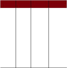
114 |
CHAPTER 5 Advanced data management |
uniquely identified by knowing that it’s from observation (ID) 1, at Time 1, and on variable X1.
MELTING
When you melt a dataset, you restructure it into a format where each measured variable is in its own row, along with the ID variables needed to uniquely identify it. If you melt the data from table 5.8, using the following code
library(reshape)
md <- melt(mydata, id=(c("id", "time")))
you end up with the structure shown in table 5.9.
Note that you |
must |
specify the |
Table 5.9 The melted dataset |
|
|||
variables needed to uniquely identify each |
|
||||||
|
|
|
|
||||
measurement (ID and Time) and that |
ID |
Time |
Variable |
Value |
|||
the variable indicating the measurement |
|
|
|
|
|||
1 |
1 |
X1 |
5 |
||||
variable names (X1 or X2) is created for |
|||||||
|
|
|
|
||||
you automatically. |
|
|
1 |
2 |
X1 |
3 |
|
Now that you have your data in a melted |
2 |
1 |
X1 |
6 |
|||
form, you can recast it into any shape, using |
|||||||
|
|
|
|
||||
the cast() function. |
|
|
2 |
2 |
X1 |
2 |
|
CASTING |
|
|
1 |
1 |
X2 |
6 |
|
The cast() function |
starts |
with melted |
1 |
2 |
X2 |
5 |
|
data and reshapes it using a formula that |
|||||||
|
|
|
|
||||
you provide and an (optional) function |
2 |
1 |
X2 |
1 |
|||
used to aggregate the data. The format is |
2 |
2 |
X2 |
4 |
|||
|
|
|
|||||
newdata <- cast(md, formula, FUN)
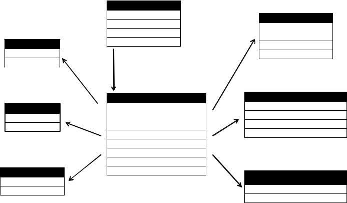
where md is the melted data, formula describes the desired end result, and FUN is the (optional) aggregating function. The formula takes the form
rowvar1 + rowvar2 + … ~ colvar1 + colvar2 + …
In this formula, rowvar1 + rowvar2 + … define the set of crossed variables that define the rows, and colvar1 + colvar2 + … define the set of crossed variables that define the columns. See the examples in figure 5.1.
Because the formulas on the right side (d, e, and f) don’t include a function, the data is reshaped. In contrast, the examples on the left side (a, b, and c) specify the mean as an aggregating function. Thus the data are not only reshaped but aggregated as well. For example, (a) gives the means on X1 and X2 averaged over time for each observation. Example (b) gives the mean scores of X1 and X2 at Time 1 and Time 2, averaged over observations. In (c) you have the mean score for each observation at Time 1 and Time 2, averaged over X1 and X2.
As you can see, the flexibility provided by the melt() and cast() functions is amazing. There are many times when you’ll have to reshape or aggregate your data prior to analysis. For example, you’ll typically need to place your data in what’s called
With Aggregation
cast(md, id~variable, mean)
ID |
X1 |
X2 |
|
|
|
1 |
4 |
5.5 |
|
|
|
2 |
4 |
2.5 |
|
|
|
(a)
cast(md, time~variable, mean)
Time X1 X2
1 5.5 3.5
2 2.5 4.5
(b)
cast(md, id~time, mean)
ID |
Time1 |
Time2 |
|
|
|
|
|
|
1 |
5.5 |
4 |
|
|
|
|
|
|
2 |
3.5 |
3 |
|
|
|
|
|
|
(c)
Reshaping a Dataset
mydata
ID |
Time |
X1 |
X2 |
|
|
|
|
|
|
|
|
1 |
1 |
5 |
6 |
|
|
|
|
|
|
|
|
1 |
2 |
3 |
5 |
|
|
|
|
|
|
|
|
2 |
1 |
6 |
1 |
|
|
|
|
|
|
|
|
2 |
2 |
2 |
4 |
|
|
|
|
|
|
|
|
md <- melt(mydata, id=c("id", "time"))
ID |
Time |
Variable |
Value |
|
|
|
|
|
|
|
|
1 |
1 |
X1 |
5 |
|
|
|
|
|
|
|
|
1 |
2 |
X1 |
3 |
|
|
|
|
|
|
|
|
2 |
1 |
X1 |
6 |
|
|
|
|
|
|
|
|
2 |
2 |
X1 |
2 |
|
|
|
|
|
|
|
|
1 |
1 |
X2 |
6 |
|
|
|
|
|
|
|
|
1 |
2 |
X2 |
5 |
|
|
|
|
|
|
|
|
2 |
1 |
X2 |
1 |
|
|
|
|
|
|
|
|
2 |
2 |
X2 |
4 |
|
|
|
|
|
|
|
|
Figure 5.1 Reshaping data with the melt() and cast() functions
Without Aggregation
cast(md, id+time~variable)
ID |
Time |
X1 |
X2 |
|
|
|
|
|
|
|
|
1 |
1 |
5 |
6 |
|
|
|
|
|
|
|
|
1 |
2 |
3 |
5 |
|
|
|
|
|
|
|
|
2 |
1 |
6 |
1 |
|
|
|
|
|
|
|
|
2 |
2 |
2 |
4 |
|
|
|
|
|
|
|
|
(d)
cast(md, id+variable~time)
ID |
Variable |
Time1 |
Time 2 |
|
|
|
|
|
|
|
|
1 |
X1 |
5 |
3 |
|
|
|
|
|
|
|
|
1 |
X2 |
6 |
5 |
|
|
|
|
|
|
|
|
2 |
X1 |
6 |
2 |
|
|
|
|
|
|
|
|
2 |
X2 |
1 |
4 |
|
|
|
|
|
|
|
|
(e)
cast(md, id~variable+time)
ID |
X1 |
X1 |
X2 |
X2 |
|
Time1 |
Time2 |
Time1 |
Time2 |
|
|
|
|
|
|
|
|
|
|
1 |
5 |
3 |
6 |
5 |
|
|
|
|
|
|
|
|
|
|
2 |
6 |
2 |
1 |
4 |
|
|
|
|
|
|
|
|
|
|
(f)
restructuring and Aggregation
115