Baer M., Billing G.D. (eds.) - The role of degenerate states in chemistry (Adv.Chem.Phys. special issue, Wiley, 2002)
.pdf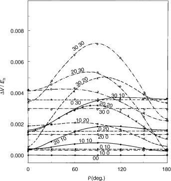
renner–teller effect and spin–orbit coupling |
637 |
Figure 9. Energy difference (absolute value) between the components of the X2 electronic state of HCCS as a function of coordinates r1; r2, and g. Curves represent the square root of the second of functions given by Eq. (77) (with e01 ¼ 0:011; e02 ¼ 0:013; e012 ¼ 0:005325) for fixed values of coordinates r1 and r2 (attached at each curve) and variable g ¼ f2 f1. Here g ¼ 0 corresponds to cis-planar geometry and g ¼ p to trans-planar geometry. Symbols: results of explicit ab initio calculations.
three-parameter formulas (75) and (77) and those actually calculated looks very satisfactory. Some significant discrepancies can be noted only at large deviations from linearity (r1 ¼ 30 ; r2 ¼ 30 ), where the harmonic approximation is not expected to be reliable.
For the variational calculations of the vibronic spectrum and the spin–orbit fine structure in the X2 state of HCCS the basis sets involving the bending functions up to u1 ¼ u2 ¼ 11 with all possible l1 and l2 values are used. This leads to the vibronic secular equations with dimensions 600 for each of the vibronic species considered. The bases of such dimensions ensure full
638 |
miljenko peric´ and sigrid d. peyerimhoff |
convergence of vibronic energies in the energy range from 0 to 2500 cm 1 with respect to the minimum of the potential surface.
Two sets of calculations for the vibronic spectrum were carried out. In the first, the zeroth-order kinetic energy operator given by Eq. (46) is employed. The second set of calculations is performed using the kinetic energy operator for large-amplitude bending with bond lengths kept constant [144]. The results of both sets of calculations do not differ from one another by more than a few wavenumbers (see [152] for a more detailed analysis) and thus we present below only those obtained using the zeroth-order kinetic energy operator.
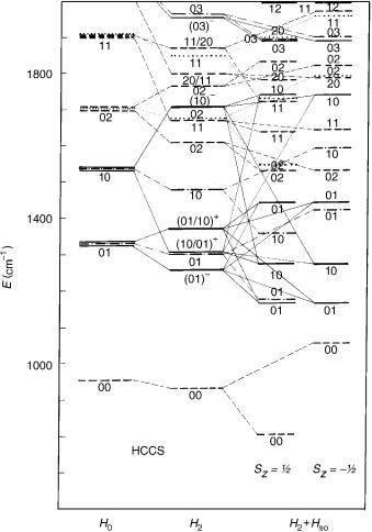
The results of calculation of the HCCS vibronic spectrum are displayed in Figure 10. Let us skip at this place from the notation used thus far (u1; l1; u2; l2) to the usual spectroscopic one, according to which the indexs 4 and 5 are employed for (predominantly) H C C and C C S bending modes, respectively. Three sets of vibronic energy levels are given: The first one represent zeroth-order values obtained by neglecting the R–T effect and the spin–orbit coupling—they correspond thus to the mean potential surface for the X2 electronic state. The second set of vibronic energy values is generated in computations in which the R–T coupling is taken into account, but the spin– orbit coupling is neglected. We present the results for K ¼ 0, 1, 2, and 3 states. The third sample of vibronic energies represents the final results obtained by including both the vibronic and spin–orbit coupling effects. In all cases the composition of the vibronic wave functions in terms of dominating basis functions (denoted by the vibrational quantum numbers u4; u5) is given. The low-lying vibronic states, computed at different levels of approximation, correlating (approximately) with one another are connected with thin lines.
Since the basis functions employed in variational calculations are not expressed in terms of the normal coordinates, the labeling of the vibronic levels by the quantum numbers u4 and u5 is approximate (so, e.g., the lowest lying K ¼ 0 vibronic state, assigned to u4 ¼ 0, u5 ¼ 1, contains an appreciable contribution from the basis function with u4 ¼ 1, u5 ¼ 2), Harmonic bending frequencies computed in the this study (o4 ¼ 579 cm 1, o5 ¼ 374 cm 1) are in very good agreement with the corresponding experimental findings (565, 380 cm 1, respectively) [139]. The spin–orbit coupling constant ( 261 cm 1) is in excellent agreement with the value extracted by Tang and Saito [139] from the experimental findings.
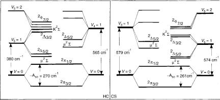
We do not wish to go into the details of Figure 10. As an illustration of the reliability of the present results we compare, however, in Figure 11, the structure of the measured HCCS spectrum published by Tang and Saito (Fig. 3 of [139]) with the results of the theoretical study. Taking into account the very complex and unusual structure of this kind of spectra, we find the agreement between our ab initio theoretical results and those following from the interpretation of experimental spectra more than satisfactory. While strongly
640 |
miljenko peric´ and sigrid d. peyerimhoff |
Figure 11. Left: Vibronic structure of the X2 state of HCCS derived by Tang and Saito from experimental findings (Fig. 3 of [139]). Right: Corresponding results of the ab initio study presented in [152].
supporting the analysis of the experimental findings, carried out by Tang and Saito, the results of the ab initio study offered a number of additional data that could be helpful in future experimental work on this subject.
V.CONCLUSION
In this chapter, we give a review of results of ab initio treatments of the R–T effect and spin–orbit coupling in triatomic and tetraatomic molecules. We have tried to present a comprehensive up to date literature survey and to compare various approaches with one another. Our prime goal was to present the development of ideas that finally resulted in those methods that are nowadays widely used to produce numerical results serving to interpret and to predict features of concrete molecular systems. A consequence of these restrictions is that we only mentioned those model treatments in which the main goal is rather to explain qualitative aspects of the vibronic coupling than to consider particular molecules, and the effective Hamiltonian approaches that do not rely on ab initio computations; we did not even mention several alternative theoretical approaches [168,169] not directly on the main stream we followed in this study. We have tried to document that the handling of the R–T effect by means of modern ab initio techniques not only offers reliable interpretation of experimental findings but also has reached the level of numerical accuracy so that it can compete with high-resolution spectroscopy.
renner–teller effect and spin–orbit coupling |
641 |
APPENDIX A: PERTURBATIVE HANDLING OF THE RENNER–TELLER EFFECT AND SPIN–ORBIT COUPLING IN ELECTRONIC STATES OF TETRAATOMIC MOLECULES
The perturbation theory has for a long time been the leading tool for handling the R–T effect in triatomic molecules (for an overview see, e.g. [8] and [12]). It was also applied in the first theoretical paper on tetraatomic molecules [132] to singlet states of both symmetric (ABBA) and asymmetric (ABCD) species. The combined effect of vibronic and spin–orbit coupling in the lowest lying vibronic species was considered by Tang and Saito [139]. Several new perturbative formulas for singlet states of symmetric tetraatomic molecules were derived in [153], and a perturbative treatment of 1 electronic states of the same molecular species was presented in [150]. In two recent studies [170,171] the present authors gave the second-order perutbative formulas for the combined effect of vibronic and spin–orbit coupling in and electronic states of triatomic and symmetric tetraatomic molecules with linear equilibrium geometry. They were derived employing two schemes for partitioning the model Hamiltonian: In the first, the term descibing the spin–orbit coupling is tretad as perturbation (together with the term responsible for vibronic interaction). In the second approach, reliable for the cases when the spin–orbit coupling constant is comparable in magnitude to the bending frequency, the spin–orbit operator is included into the zeroth-order Hamiltonian. In this chapter, we give only the formula obtained via the first scheme. Moreover, we restrict ourselves to tetraatomic molecules, because the perturbative formulas for triatomics can be looked upon as special cases of their counterparts for tetraatomic species.
The perturbative handling of the R–T effect in molecules with more than three atoms is much more complicated than that for triatomics, because of the presence of more than one bending mode contributing to the vibronic interaction. A consequence is that the perturbative formulas cannot be derived for a general case, because the level of degeneracy of zeroth-order vibronic levels increases rapidly with increasing values for the bending quantum numbers (in the case of triatomics all zeroth-order vibronic levels are either nondegenerate or twofold degenerate).
The present perturbative treatment is carried out in the framework of the minimal model we defined above. All effects that do not crucially influence the vibronic and fine (spin–orbit) structure of spectra are neglected. The kinetic energy operator for infinitesimal vibrations [Eq. (49)] is employed and the bending potential curves are represented by the lowest order (quadratic) polynomial expansions in the bending coordinates. The spin–orbit operator is taken in the phenomenological form [Eq. (16)]. We employ as basis functions

renner–teller effect and spin–orbit coupling |
643 |
angular momentum caused by the 2D trans and cis bending vibrations, respectively. Their algebraic sum with the electronic angular quantum number gives
the good (in the framework |
of |
the |
present |
model) |
quantum |
number |
K; K ¼ lT þ lC ¼ lT0 þ lC0 þ |
. |
The |
sum of |
K and |
the spin |
quantum |
number results in the quantum number for the projection of the total angular momentum along the molecular axis, P ¼ K þ .
The perturbative part of the effective Hamiltonian is of the form
|
1 |
eT oT qT2 ðe 2ifT þ e2ifT Þ þ |
1 |
eCoCqC2 ðe 2ifC þ e2ifC |
|
|||
H0 ¼ |
|
|
|
Þ Aso ðA:5Þ |
||||
2 |
2 |
|||||||
We introduce for the basis functions the notation |
|
|||||||
|
1 |
1 |
|
|
|
|
||
juT lT uC lC i p2p eilT fT p2p eilC fC RuT ;lT ðqT ÞRuC ;lC ðqCÞ lT þ lC ¼ K þ |
||||||||
juT |
lT uC lC þi p eilT fT p eilC fC RuT ;lT ðqT ÞRuC ;lC ðqCÞ |
lT þ lC ¼ K |
||||||
|
1 |
1 |
|
|
|
ðA:6Þ |
||
|
|
|
|
|
|
|
|
|
|
|
|
2p |
2p |
|
|
|
|
The |
zeroth-order Hamiltonian |
and |
|
the spin–orbit part of |
the perturbation |
|||
are diagonal with respect to the quantum numbers K; ; P; uT ; lT ; uC and lC. The
matrix elements h lC uC lT uT jH0juT0 lT0 |
uC0 lC0 þi of the remaining part of the |
||||
perturbative operator can be different |
from zero only if lT0 ¼ lT 2; |
uT0 ¼ |
|||
uT ; uT 2; lC0 |
¼ lC; uC0 ¼ uC, or lT0 ¼ lT ; uT0 |
¼ uT ; lC0 |
¼ lC 2; uC0 |
¼ uC; |
|
uC 2. These |
selection rules automatically |
comprise |
the g/u symmetry |
||
restrictions.
As mentioned above, as a consequence of the fact that the degeneracy of the zeroth-order vibronic levels in tetraatomic molecules increases rapidly with increasing value of the bending quantum numbers uT and uC [it is equal to 2ð2uT þ 1Þð2uC þ 1Þ if spin is neglected] and thus the secular equations to be solved in the framework of the perturbation theory are multidimensional, only several special coupling cases can be handled efficiently. We present here those for which the dimension of the secular equation is effectively not larger than 2; however, some other cases can also be handled, particularly if the spin–orbit coupling is relatively large compared to the separation of the electronic states at relevant bent geometries.
Case Aa uT 6¼ 0; uC ¼ 0
In this case, the situation is essentially equivalent to that for triatomics molecules. (We shall always assume that uT uC; the formulas for the opposite case, uT uC, are obtained from those to be derived by interchanging simply