

Signal Processing of Random Physiological Signals - Charles S. Lessard
.pdf71
C H A P T E R 9
Correlation Functions
In the general theory of harmonic analysis, an expression of considerable importance and interest is the correlation function given in (9.1).
1 |
T1/2 |
|
|
f1(t) f2(t + τ )d t |
(9.1) |
||
T |
−T1/2
For the case of periodic functions where f1(t) and f2(t) have the same fundamental angular frequency ω1 and where τ is a continuous time of displacement in the range (−∞ , ∞), independent of t (the ongoing time).
One important property of the correlation expression is the fact that its Fourier Tra-
nsform is given by (9.2), where f1(t) has the complex spectrum F1(n), and |
f2(t) has F2(n). |
||
|
|
(n)F2(n) |
(9.2) |
|
F1 |
||
The bar (F1(n)) indicates the complex conjugate of the quantity (function) over which it is placed. To establish this fact, the Fourier expansion of f1(t) and f2(t) can be expressed as (9.3) and (9.4).
f1(t) = |
∞ |
|
F1(n)e j nω1t |
(9.3) |
|
|
n=−∞ |
|
f2(t) = |
∞ |
|
F2(n)e j nω1t |
(9.4) |
n=−∞
where the complex spectrums are given by (9.5) and (9.6), respectively.
|
1 |
T1/2 |
|
|
F1(n) = |
f1(t)e − j nω1t d t |
(9.5) |
||
T1 |
−T1/2

72 SIGNAL PROCESSING OF RANDOM PHYSIOLOGICAL SIGNALS
and
|
1 |
T1/2 |
|
|
F2(n) = |
f2(t)e − j nω1t d t |
(9.6) |
||
T1 |
−T1/2
However, it should be noted from (9.1) that the original equation is not for f2(t) but rather for f2(t + τ ). Thus, it was found that caution must be taken in the manner that the correlation function is expressed:
1 |
T1/2 |
|
1 |
T1/2 |
∞ |
|
||||
|
|
|
|
f1(t) f2(t + τ )d t = |
|
|
|
f1(t)d t |
F2(n)e j nω1(t+τ ) |
(9.7) |
T |
|
|
T |
|
||||||
|
−T1 |
/ |
2 |
|
|
−T1 |
/ |
2 |
n=−∞ |
|
|
|
|
|
|
|
|
||||
The manner in which the right-hand side of the equation is written indicates that summation with respect to n comes first and is followed by integration with respect to t, as shown in (9.7).
At this point, if the order of summation and integration is inversed, the result would be given by (9.8):
1 |
T1/2 |
∞ |
1 |
T1/2 |
|
||||
|
|
|
f1(t) f2(t + τ )d t = |
F2(n)e j nω1τ |
|
|
|
f1(t)e j nω1t d t |
(9.8) |
T1 |
/ |
T1 |
/ |
||||||
|
−T1 |
2 |
n=−∞ |
|
−T1 |
2 |
|
||
|
|
|
|
|
|
||||
Note that in (9.8), the exponent in the second term (the integral) has a positive, + j , rather than a negative, − j , as shown in the integral ( d t) of (9.5), where the last integral is recognized as the complex conjugate of F1(n). Hence, the result yields (9.10),
1 |
T1/2 |
∞ |
|
|
|
||
|
|
|
|
|
|
||
|
|
|
f1(t) f2(t + τ )d t = |
[F1(n)F2(n)]e j nω1τ |
(9.10) |
||
T1 |
/ |
||||||
|
−T1 |
2 |
n=−∞ |
|
|||
|
|
|
|
|
|
||
which results in the general form of the inverse Fourier Transform (9.11) for a periodic function of fundamental angular frequency ω1 and complex spectrum F1(n)F2(n) of (9.10).
f (t) = |
∞ |
|
F (n)e j n 1t |
(9.11) |
n=−∞
However, note that (9.10) is in terms of delays, τ , instead of time, t, as in (9.11). Then

CORRELATION FUNCTIONS 73
by applying the definition of the Fourier Transform of the periodic function f (t) as in (9.12),
|
1 |
T1/2 |
|
|
F (n) = |
f (t)e − j nω1t dt for n = 0, ±1, ±2, ±. . . . |
(9.12) |
||
T1 |
−T1/2
and substituting the convolution function for f (t) as in (9.13):
1 |
T1/2 |
|
|
f1(t) f2(t + τ )d t = f (t) |
(9.13) |
||
T |
−T1/2
the complex spectrum F1(n)F2(n) becomes (9.14):
|
|
1 |
T1/2 |
T1/2 |
|
|
|
|
e − j nω1τ d τ |
|
|
||
F1(n)F2(n) = |
f1(t) f2(t + τ )d t |
(9.14) |
||||
|
||||||
T1 |
||||||
|
|
|
−T1/2 |
−T1/2 |
|
|
Again, the right integration is preformed first with respect to t and the resulting function of τ is then multiplied by e − j nω1τ . Then, the product is integrated with respect
to τ in order to obtain a function of n.
Thus the equations in (9.15) are Fourier Transforms of each other.
1 |
T1/2 |
|
|
f1(t) f2(t + τ )dt and F1(n)F2(n) |
(9.15) |
||
T1 |
−T1/2
This relationship is called the “Correlation Theorem” for periodic functions.
9.1THE CORRELATION PROCESS
The correlation process involves three important operations:
(1)The periodic function f2(t) is given as delays or time displacement, τ .
(2)The displacement function is multiplied by the other periodic function of the same fundamental frequency.
(3)The product is averaged by integration over a complete period.
These steps are repeated for every value τ in the interval (−∞, ∞) so that a function
is generated. In summary, the combination of the three operations—displacement,

74 SIGNAL PROCESSING OF RANDOM PHYSIOLOGICAL SIGNALS
multiplication, and integration—are termed “Correlation,” whereas folding, displacement, multiplication, and integration are referred to as “Convolution,” a totally different process. Correlation is not limited to periodic functions, as it can be applied to aperiodic and random functions.
9.1.1 Autocorrelation Function
Basic statistical properties of importance in describing single stationary random processes include autocorrelation functions and autospectral density functions. In the correlation theorem for periodic functions, it was found that under the special conditions, the two functions may be identical, f1(t) = f2(t). In this case, the correlation equation becomes (9.16) and is referred to as the “Autocorrelation Function.”
1 |
T1/2 |
∞ |
|
|
|
|
||
|
|
|
|
2 |
e j nω1τ |
|
||
|
|
|
|
|
||||
|
|
|
|
f1(t) f1(t + τ )d t = |
|F1(n)| |
(9.16) |
||
T1 |
/ |
|
||||||
|
−T1 |
2 |
n=−∞ |
|
|
|
|
|
|
|
|
|
|
|
|
||
For the case in which τ = 0, it means that the squared value of the function f1(t) is equal to the sum of the squares of the absolute values over the entire range of harmonics in the spectrum of the function. Because the expression on the left divides the integrated results, the autocorrelation at zero delay is referred to as the Mean Squared Value of the function. The autocorrelation function is often subscripted as ϕ11 in the time domain or as Φ11 in the frequency domain. The reciprocal relations expressed in (9.17) and (9.18) form the basis for the “Autocorrelation Theorem” for periodic functions.
Expressed in words, the theorem states that the autocorrelation function and the power spectrum of a periodic function are “Fourier” transforms of each other. Equation (9.17) is the time domain expression, stating that the autocorrelation is equal to the
“Inverse Fourier” transform of the power spectrum.
ϕ11(τ ) = |
∞ |
|
11(n)e j nω1τ |
(9.17) |
n=−∞
Equation (9.18) is the frequency domain expression, stating that the “Fourier” transform of the autocorrelation function is equal to the power spectrum of the function.
|
T1 |
|
|
|
11(n) = |
2 |
ϕ11e − j nω1τ d τ |
(9.18) |
|
|
T1 |
|||
− |
|
|
|
|
2 |
|
|
||

CORRELATION FUNCTIONS 75
9.2PROPERTIES OF THE AUTOCORRELATION FUNCTION
One of the properties of an autocorrelation function is that although it retains all harmonics of the given function, it discards all their phase angles. In other words, all periodic functions having the same harmonic amplitudes but differing in their initial phase angles have the same autocorrelation function or that the power spectrum of a periodic function is independent of the phase angles of the harmonics.
Another important property is that the autocorrelation function is an Even Function of τ . An even periodic function satisfies the expression given by (9.20).
ϕ11(−τ ) = ϕ11(τ ) |
(9.20) |
The proof is as follows: writing (9.16) as a function of a negative delay, −τ , gives (9.21).
|
1 |
T1/2 |
|
|
ϕ11(−τ ) = |
f1(t) f1(t − τ )d t |
(9.21) |
||
|
||||
T1 |
||||
|
|
−T1/2 |
|
Using the change of variable, since x = (t − τ ) or x = (t + τ ), then the limits become T1/2 − τ ; −T1/2 − τ , and f1(t − τ ) becomes f1(x + τ − τ ) = f1(x). Likewise, f1(t) becomes f1(t + τ ). Also since ϕ11(τ ) is a periodic function of period T1, integration over the interval, −T1/2 − τ to T1/2 − τ , is the same as T1/2 to −T1/2. The result is 9.22:
|
1 |
T1/2 |
|
|
ϕ11(−τ ) = |
f1(t) f1(t + τ )d t or that ϕ11(−τ ) = ϕ11(τ ) |
(9.22) |
||
T1 |
−T1/2
9.3STEPS IN THE AUTOCORRELATION PROCESS
The autocorrelation process requires the five steps listed as follows:
1.Change of variable from time (t) to delay (τ )
2.Negative translation along the horizontal x-axis (N is the total number of delays)
76SIGNAL PROCESSING OF RANDOM PHYSIOLOGICAL SIGNALS
3.Positive incremental translation along the horizontal x-axis (one delay)
4.Multiplication of the two functions, f1(τ ) and f2(t − τ )
5.Integration of area
Steps 3 through 5 are repeated until 2N delays are completed
The process might be synopsized as determining the area under the curves (product) as the folded function is slid along the horizontal axis. Note the direction of translation; the conventional notation is as follows:
a.Movement to the right for positive (+) time
b.Movement to the left for negative (−) time
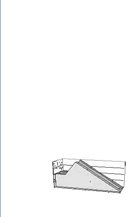
At this point, let us go through an example to visualize the autocorrelation process. The function f1 is shown in Fig. 9.1 as two repeated graphs. To simplify the example, the change of variable will not be preformed or shown.
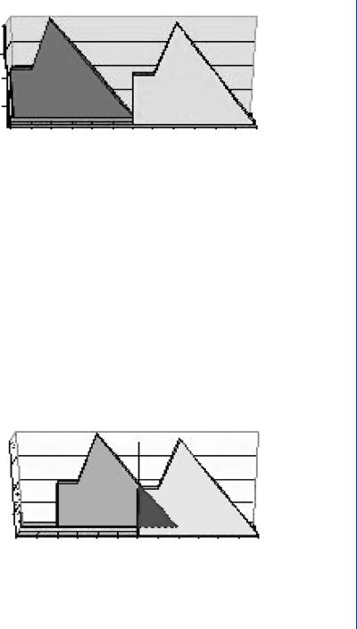
The second step is to translate or move one of the functions in the negative direction without reversing the function. Figure 9.2 shows what the graph of the two functions would look like. Note that x = 0 is in the middle of the axis.
The next step is that of moving the translated function in a positive direction by 2 delays (from 0 to +2) along the x-axis as shown in Fig. 9.3. Note that the overlapping area is the area of both functions between 0 and +2 on the x-axis.
Autocorrelation first step
Magnitude
2 |
|
|
|
|
|
|
1.5 |
|
|
|
|
|
|
1 |
|
|
|
|
|
|
0.5 |
|
Original f |
|
|
|
|
0 |
|
|
|
|
|
|
0 |
1 |
2 |
3 |
4 |
|
|
|
|
5 |
6 |
|||
|
|
|
Time (t) |
|
||
|
|
|
|
|
|
|
FIGURE 9.1: Starting the autocorrelation process. The function f1 is shown as two separate 3-D objects
CORRELATION FUNCTIONS 77
Autocorrelation direct translation
2
Magnitude
1.5
1
0.5
f1
0 |
|
|
|
|
|
|
|
|
|
|
|
S1 |
|
|
|
|
|
|
|
|
|
|
|
|
|
–6 |
–5 |
–4 |
–3 |
–2 |
–1 |
0 |
1 |
2 |
3 |
4 |
5 |
6 |
Time (t)
FIGURE 9.2: Step 2: Translation. Negative translation of function along the x-axis
9.4NUMERICAL CORRELATION: DIRECT CALCULATION
9.4.1 Strips of Paper Method
One of the numerical methods is to use two strips of paper in the following steps:
1.Tabulate values of the function at equally spaced intervals on two strips of paper
2.Reverse tabulate one function; f (−λ), which is equivalent to folding a function
Autocorrelation 2 Positive Shift of f 
2
Magnitude
1.5
1
0.5 |
|
|
f1 |
|
|
|
|
|
f1 |
|
|
|
|
|
|
|
|
|
|
|
|
|
|
||
0 |
–5 |
–4 |
–3 |
–2 |
–1 |
0 |
1 |
2 |
3 |
4 |
5 |
6 |
–6 |
Time (t)
FIGURE 9.3: Positive translation. The second function is moved in a positive direction by 2
delays along the x-axis. Note the overlapping area of both functions between 0 and +2 on the
x-axis

78SIGNAL PROCESSING OF RANDOM PHYSIOLOGICAL SIGNALS
3.Place strips beside each other and multiply across the strips and write the products
4.Slide one strip, and repeat step 3, until there are no more products
5.Sum the rows
6.Multiply each sum by the interval width
9.4.2 Polynomial Multiplication Method
Another method is the polynomial multiplication method (Table 9.1). For this method, the values of the function are written twice in two rows; one function is placed above the other (reverse tabulated the second time the function is written) as in Table 9.1. It should be noted that the functions are aligned as in normal multiplication; from right to left. Reverse tabulation of the second function is important; otherwise, an
TABLE 9.1: Autocorrelation by Multiplication Method Correct Answer
|
|
|
|
t |
|
0 |
1 |
2 |
3 |
4 |
5 |
6 |
|
|
f1 |
D |
T |
|
1 |
1 |
2 |
1.5 |
1 |
0.5 |
0 |
|
|
f1 |
R |
T |
|
0 |
0.5 |
1 |
1.5 |
2 |
1 |
1 |
|
|
|
|
|
|
|
|
|
|
|
|
|
|
|
|
|
|
|
1 |
1 |
2 |
1.5 |
1 |
0.5 |
0 |
|
|
|
|
|
1 |
1 |
2 |
1.5 |
1 |
0.5 |
0 |
|
|
|
|
|
2 |
2 |
4 |
3 |
2 |
1 |
0 |
|
|
|
|
|
1.5 |
1.5 |
3 |
2.3 |
1.5 |
0.8 |
0 |
|
|
|
|
|
1 |
1 |
2 |
1.5 |
1 |
0.5 |
0 |
|
|
|
|
|
0.5 |
0.5 |
1 |
0.8 |
0.5 |
0.3 |
0 |
|
|
|
|
|
0 |
0 |
0 |
0 |
0 |
0 |
0 |
|
|
|
|
|
|
|
|
|
|
|
|
|
|
|
|
|
|
|
0 |
0.5 |
1.5 |
3.5 |
6.3 |
8 |
9.5 |
8 |
6.3 |
3.5 |
1.5 |
0.5 |
0 |
Note: Original function ( f1); Time t ; DT is Direct Transcription; and RT is Reverse Transcription.
CORRELATION FUNCTIONS 79
TABLE 9.2: Autocorrelation by Multiplication Method Incorrect Answer
|
|
|
t |
|
|
0 |
1 |
2 |
3 |
4 |
5 |
6 |
|
|
f1 |
D |
T |
|
1 |
1 |
2 |
1.5 |
1 |
0.5 |
0 |
|
|
f1 |
D |
T |
|
1 |
1 |
2 |
1.5 |
1 |
0.5 |
0 |
|
|
|
|
|
|
0 |
0 |
0 |
0 |
0 |
0 |
0 |
|
|
|
|
|
0.5 |
0.5 |
1 |
0.8 |
0.5 |
0.3 |
0 |
|
|
|
|
|
1 |
1 |
2 |
1.5 |
1 |
0.5 |
0 |
|
|
|
|
|
1.5 |
1.5 |
3 |
2.3 |
1.5 |
0.8 |
0 |
|
|
|
|
|
2 |
2 |
4 |
3 |
2 |
1 |
0 |
|
|
|
|
|
1 |
1 |
2 |
1.5 |
1 |
0.5 |
0 |
|
|
|
|
|
1 |
1 |
2 |
1.5 |
1 |
0.5 |
0 |
|
|
|
|
|
|
|
|
|
|
|
|
|
|
|
|
|
|
|
1 |
2 |
5 |
7 |
9 |
9 |
7.3 |
5 |
2.5 |
1 |
0.3 |
0 |
0 |
|
|
|
|
|
|
|
|
|
|
|
|
|
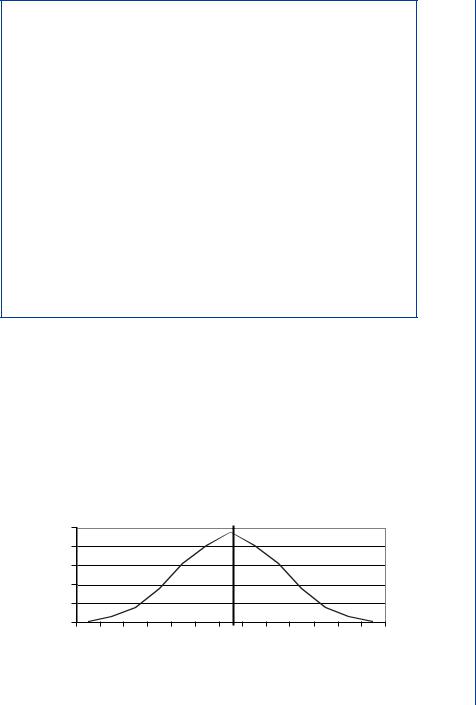
incorrect answer is obtained as shown in the calculations of Table 9.2. The number of terms in the results should equal twice the number of terms in the function. The final results of the correlation operation are obtained by summing the column and multiplying by the interval width. The graph of the correct calculation is shown in Fig. 9.4; note that the autocorrelation function is an even function (symmetrical about the y -axis).
Magnitude |
10 |
|
8 |
||
6 |
||
4 |
||
2 |
||
|
||
|
0 |
|
|
-6 -5 -4 -3 -2 -1 0 1 2 3 4 5 6 |
|
|
Time (t ) |
FIGURE 9.4: Correct calculation of autocorrelation. The graph shows the result of Table 9.1
calculations. Note that the autocorrelation function is an even function

80 SIGNAL PROCESSING OF RANDOM PHYSIOLOGICAL SIGNALS
|
10 |
|
|
|
|
|
|
|
|
|
|
|
|
Magnitude |
8 |
|
|
|
|
|
|
|
|
|
|
|
|
6 |
|
|
|
|
|
|
|
|
|
|
|
|
|
4 |
|
|
|
|
|
|
|
|
|
|
|
|
|
2 |
|
|
|
|
|
|
|
|
|
|
|
|
|
|
|
|
|
|
|
|
|
|
|
|
|
|
|
|
0 |
|
|
|
|
|
|
|
|
|
|
|
|
|
6 |
5 |
4 |
3 |
2 |
1 |
0 |
1 |
2 |
3 |
4 |
5 |
6 |
|
|
|
|
|
|
Time (t ) |
|
|
|
|
|
||
FIGURE 9.5: Incorrect autocorrelation results. Note the lack of symmetry in the graph of the
incorrect calculation results of Table 9.2
For the Direct Numerical Method via polynomial multiplication, use the following
steps:
1.directly tabulate values of the function in the second row with the increment of time above the function as in Table 9.1;
2.reverse tabulate the same function in the third row;
3.do normal polynomial multiplication (from right to left);
4.write the products in columns following normal multiplication procedures;
5.when there are no more products, sum the columns; and
6.multiply each sum by the interval width.
It is important to “Reverse tabulate” the second function; otherwise, the incorrect answer is obtained as shown in the calculations of Table 9.2. The graph of the incorrect results is shown in Fig. 9.5. Note the lack of symmetry.
9.5CROSS-CORRELATION FUNCTION
For pairs of random data from two different stationary random processes, the joint statistics of importance include the cross-correlation and cross-spectral density functions. The cross-correlation theorem for periodic functions f1(t) and f2(t) applies to two different periodic functions, but with the stipulation that the functions must have the