

Signal Processing of Random Physiological Signals - Charles S. Lessard
.pdfCORRELATION FUNCTIONS 81
same fundamental frequency. If the condition of the same fundamental frequency is met, the cross-correlation function is defined as given by (9.23) for continuous data or by (9.24) for discrete data,
|
|
|
1 |
T1/2 |
|
|||
ϕ12(τ ) = |
f1(τ ) f2(t + τ )d t |
(9.23) |
||||||
|
||||||||
T1 |
||||||||
|
1 |
n |
|
−T1/2 |
|
|||
|
|
|
|
|
|
|||
rx y (τ ) = |
|
xi (t) yt (t + τ ) = x(t)y (t + τ ) |
(9.24) |
|||||
|
|
|||||||
N |
i =1 |
|||||||
|
|
|
|
|
|
|
||
and cross-power spectrum of the functions as (9.25).
|
|
|
|
12(n) = F1(n)F2(n) |
(9.25) |
||
The subscripts 12 indicate that the cross-correlation involves f1(t) and f2(t) with the second numeral (2) referring to the fact that f2(t) has the displacement τ .
It is important to keep the numerals in the double subscripts in proper order; because, if we interchange the order of the subscripts, then by definition the resulting cross-correlation function is given by (9.26).
|
1 |
T1/2 |
|
|
ϕ21(τ ) = |
f2(τ ) f1(t + τ )d t |
(9.26) |
||
T1 |
−T1/2
Some text books will use the notation, Rx y , which is referred to as the correlation of x with y . The correlation of y with x is then expressed as (9.27). Note that the first subscript in either equation is the function without (t + τ ). The preferred equation for the cross-correlation expression is (9.26).
∞ |
|
Ry x = x(t + τ )y (t)d τ |
(9.27) |
0
The subscripts for the cross-spectrum are given in (9.28); note that the conjugated function is the first subscript.
|
|
|
|
21(n) = F2(n)F1(n) |
(9.28) |
||
The importance of keeping the numerals in the double subscript in the proper order
82 SIGNAL PROCESSING OF RANDOM PHYSIOLOGICAL SIGNALS
0.2
R12: Cross correlation
0.1
0.0
–0.1
–0.2
–0.8 |
–0.6 |
–0.4 |
–0.2 |
0.0 |
0.2 |
0.4 |
0.6 |
0.8 |
1.0 |
0.2
R21: Cross correlation
0.1
0.0
–0.1
–0.2
–0.8 |
–0.6 |
–0.4 |
–0.2 |
0.0 |
0.2 |
0.4 |
0.6 |
0.8 |
1.0 |
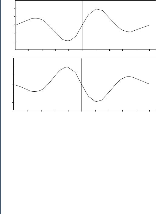
FIGURE 9.6: Cross-correlation |
images. |
The |
graphs show |
the |
comparison |
of |
the cross- |
||
correlation function 12(n)[R12] to its complex conjugate image 21(n)[R21]
can not be overstressed. If the subscripts are interchanged, the results will not be what is expected. This interchange can be made by changing +τ in the definition to −τ and letting x = t − τ , leading to the expression (9.29). The fact is that ϕ12(−τ ) is the mirror image of ϕ21(τ ) with respect to the vertical axis.
ϕ12(−τ ) = ϕ21(τ ) |
(9.29) |
The representation of the property in the frequency domain is given by (9.30).
12(n) = |
|
21 (n) |
(9.30) |
In summary, 12(n) and 21(n) are related to each other as complex conjugate quantities. Figure 9.6 shows the graphs comparing the cross-correlation function 12(n)[R12] to its complex conjugate image 21(n)[R21].

CORRELATION FUNCTIONS 83
9.5.1 Properties of the Cross-Correlation Function
The cross-correlation function possesses several properties which are valuable in appli-
cations to signal and data processing:
1.Rx y (τ ) = Rx y (−τ ) The cross-correlation is not an “Even Function.”
2.Rx y (τ ) ≤ Rx y (0)Ry x (0) = x2 y 2(the product of the RMS values of x and y )
3.If x and y are independent variables, then
Rx y (0) = Ry x (0) = x y (the product of the mean values of x and y )
4.If x and y are both periodic with period = T0, then Rx y and Ry x are also periodic with period = T0.
5.The cross-power spectrum of x and y is computed as the Fourier Transform of the cross-correlation function.
9.5.2Applications of the Cross-Correlation Function
1.An indication of the predictive power of x to y (or vice versa) is given by the magnitude of the correlation function. Delays of the effects of x on y are indicated by the value of t at which Rx y reaches a maximum.
2.The RMS and mean values of x or y can be estimated through the use of properties 2 and 3 given above, provided that the values of one function are known.
3.Periodicities in x and y can be detected in the cross-correlation function (Property 4).
4.The cross-power spectrum, given by the Fourier transform of the crosscorrelation, is used in the calculation of the coherence of the functions.

85
C H A P T E R 1 0
Convolution
The convolution integral dates back to 1833. It is one of the methods used to determine the output response of a system to a specific input if the system transfer function is known. Convolution applies the superposition principal. Conceptually,
1.the input signal is represented as a continuum of impulses;
2.the response of the system to a single impulse is obtained;
3.the response of the system to each of the elementary impulses, representing the input, is computed; and then
4.the total input response is obtained by superposition.
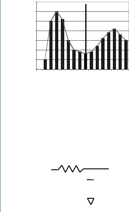
Often signals are represented in terms of elementary linear basis functions, but not as a continuum of impulses. Therefore let us examine the representation of an arbitrary time function by a continuum of impulses. Let us begin with the approximation of a function f (t) in the interval −T to +T by rectangles (rectangular pulses) whose height is equal to the function at the center of the rectangular pulse, and the width is T
(Fig. 10.1).
The equation describing the impulse representation of the continuous signal is given by (10.1).
f (t) = |
+T |
|
f (τ )δ (t − τ ) ∂ τ from − T < t < T |
(10.1) |
|
|
−T |
|
Since the convolution is used in the time domain analysis of a filter response, let us
86 SIGNAL PROCESSING OF RANDOM PHYSIOLOGICAL SIGNALS
3.5 |
Y |
3 |
2.5 |
2 |
1.5 |
1 |
0.5 |
0 |
–T –7 –6 –5 –4 –3 –2 –1 0 1 2 3 4 5 6 7 T |
FIGURE 10.1: A signal represented in terms of a continuum of impulses in the interval,
−T to +T
examine how the convolution integral is used to obtain the system impulse response of a simple RC circuit or low pass filter as shown in Fig. 10.2.
If a single unit pulse of width T and amplitude 1/T is applied, the output
voltage increases exponentially toward the value 1/T; when the pulse terminates at
T, the output voltage decays toward zero as shown in Fig. 10.3.
If the impulse is taken to its limit as t 0, then the impulse ap-
proaches a theoretical impulse; the delta function, δ, and the response to the impulse
|
R |
|||
vi(t) |
|
|
|
v0(t) |
|
|
|||
|
|
|
|
C |
|
|
|
|
|
|
|
|
|
|
FIGURE 10.2: Low-pass RC filter circuit

CONVOLUTION 87
Input: Impulse |
Filter Response |
a & b Combined |
1/ t
t
 t
t
(a) |
(b) |
(c) |
FIGURE 10.3: Low-pass filter response. (a) It shows a single unity pulse of t duration and 1/t magnitude. (b) It shows the output response of the low-pass filter shown in Fig. 10.2 to the input pulse, (a). (c) It shows the combined input and output signals
becomes (10.2).
h (t) = |
1 |
e − |
t |
(10.2) |
|
RC |
|||
RC |
What Fig. 10.4 implies is that at the instant the impulse occurs a current flows in the circuit and is supposed to charge the capacitor to a voltage of 1/RC, instantaneously. However, the instantaneous charging that theoretically occurs in the instant that the impulse is applied is not physically possible because of the principle of conservation of momentum. As a note of information, the LaPlace transformation of the delta function,
δ, is unity (1); therefore, the frequency domain is a better and easier method by which to analyze the response to an impulse function.
It is important to understand the time/frequency relationships that exist when functions are transformed into another domain. For example, the product (or Modulation)
h(t )
FIGURE 10.4: Low-pass filter response to a delta function as t 0

88 SIGNAL PROCESSING OF RANDOM PHYSIOLOGICAL SIGNALS
of two functions in the time domain corresponds to convolution in the frequency domain as shown in (10.3).
|
1 |
∞ |
1 |
|
(10.3) |
|
f1 (t) f2 (t) = |
F1 (ζ ) F2 (ω − ζ ) ∂ ζ = |
F1 (ω) × F2 (ω) |
||||
|
|
|||||
2π |
2π |
−∞
Whereas convolution in the time domain corresponds to product in the frequency domain as shown by (10.4.)
∞
f1 (t) × f2 (t) = f1 (λ) f2 (t − λ) ∂ λ F1 (ω) F2 (ω) |
(10.4) |
−∞ |
|
Convolution is commutative for time-invariant systems are given by (10.5) and (10.6).
|
∞ |
(10.5) |
y (t) = |
h (λ)x (t − λ) ∂ λ |
|
|
−∞ |
|
|
∞ |
(10.6) |
y (t) = |
x (λ)h (t − λ) ∂ λ |
−∞
Often, the convolution operation is denoted by an asterisk as shown in (10.7).
∞
f1 (t) × f2 (t) = |
f1 (λ) f2 (t − λ) ∂ λ |
(10.7) |
|
−∞ |
|
The integration limits vary with the particular characteristics of the functions being convolved. Next, let us examine and discuss the manner of “Evaluation and Interpretation of Convolution Integrals and Numerical Convolution.”
10.1CONVOLUTION EVALUATION
Formally the convolution operation is given as in (10.8).
∞
f3 = f1 × f2 = f1 (λ) f2 (t − λ) ∂ λ |
(10.8) |
−∞ |
|
CONVOLUTION 89
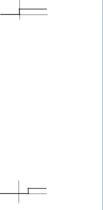
u(t)
0 t
FIGURE 10.5: Unit step function, u(t). The step function is similar to throwing a switch
The value f3 for any particular instant of time t is the area under the product of f1(λ) and f2(t − λ). To use the convolution technique efficiently, one should be able to visualize the two functions. If convolution is a new topic to the reader, then a quick review of wave form synthesis is essential for visualization. Let us begin with a step function, u(t), which is initiated at t = 0 (Fig. 10.5).
Figure 10.6 shows the unit step function translated, u(t − a ), along the time axis,
+t, by some length, +a , whereas Fig. 10.7 shows the unit step function translated backward along the time axis, −t, by some length, −a .
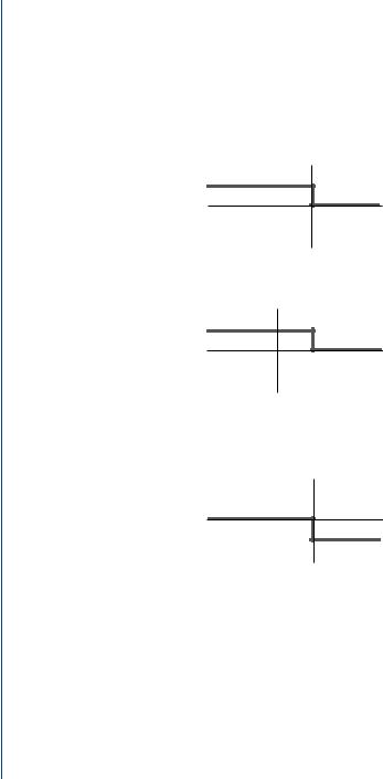
In addition, the unit step function may be rotated about the y-axis, which is referred to as folding about some axis. A folded (flipped) unit step function about the y-axis is written as, u(−t), and is shown in Fig. 10.8.
Figure 10.9 shows the result of positive translation of a folded unit step function. Note that this function is written as, u(a − t).
In addition to rotation about the y-axis, the unit step function may also be folded about the x-axis as shown in Fig. 10.10; note the negative sign in front of the unit step function, −u(t).
Figure 10.11 shows the translation of a unit step function folded about the x-axis displaced by some time value, a. This step function is written as −u(t − a ); note the negative signs.
u(t – a)
a +t
FIGURE 10.6: Positive translation. The unit step function of Fig. 10.5 is translated along the
time axis, +t, by some length, +a
90 SIGNAL PROCESSING OF RANDOM PHYSIOLOGICAL SIGNALS
|
|
|
|
|
|
|
|
u(t+a) |
|
|
|
0 |
|
|
|
-a |
t |
|
|
|
|
|
|
|
FIGURE 10.7: Negative translation. The unit step function, u(t + a ), translated backward along the time-axis, −t, by some length, −a
u(-t)
0 t
FIGURE 10.8: Folding. A unit step function rotated about the y -axis, u(−t)
u(a - t)
0 |
a |
t |
FIGURE 10.9: Positive translation of folded step function. Shown is the result of a positive translation in time (length, +a) of a folded unit step function, u(a − t)
0 t
-u(t)
FIGURE 10.10: Folding about the x-axis. A unit step function is shown folded about the x-axis,
−u(t)
|
|
a |
|
||
|
0 |
|
|
t |
|
|
|
|
-u(t - a) |
||
|
|
|
|
|
|
FIGURE 10.11: Folding and translation about the x-axis. A unit step function folded about the x-axis, t, then translated or displaced by some time value, +a