Signal Processing of Random Physiological Signals - Charles S. Lessard

132 SIGNAL PROCESSING OF RANDOM PHYSIOLOGICAL SIGNALS

FIGURE 12.6: Square waveform for example problem

By inspection, the average value over one period is zero so that a0 = 0. Value of a1 with n = 1 is

134 SIGNAL PROCESSING OF RANDOM PHYSIOLOGICAL SIGNALS

If you continue this process for other integers of n, you will obtain bn = 0 for all values of n.

Before moving into Discrete and Fast Fourier transformations and frequencydomain analysis, let me regress into perhaps the most important function to engineers, physicists, and mathematicians—the exponential function—which has the property

that the derivative and integral yield a function proportional to itself as in (12.10).

It turns out that every function or waveform encountered in practice can always be expressed as a sum of various exponential functions.

12.5 EULER EXPANSION

Euler showed that the expression, s = − j ω, of a complex frequency represents signals oscillating at angular frequency, ω, and that the cos ωt could thereby then be represented as (12.11).

e j ωt + e − j ωt

(12.11)

2

In a way, the Discrete Fourier Series is a method of representing periodic sig-

nals by exponentials whose frequencies lie along the j ω axis. Expressing the Fourier Trigonometric Series in an equivalent form in terms of exponentials, or e ± j nωt :

136 SIGNAL PROCESSING OF RANDOM PHYSIOLOGICAL SIGNALS

Fourier Transform representation of f (t). Consider the following nonperiodic signal, f (t), which one would like to represent by eternal exponential functions. As a result, we can construct a new periodic function, fT (t), with period T, where the function f (t) is represented every T seconds. The period, T, must be large enough so there is not any overlap between pulse shapes of f (t). The new function is a periodic function and can be represented with an exponential Fourier Series.

12.7 LIMITING PROCESS

What happens if the interval, T, becomes infinite for a pulse function, f (t)? Do the pulses repeat after an infinite interval? Such that fT (t) and f (t) are identical in the limit, and the Fourier Series representing the periodic function, fT (t), will also represent f (t)?

Discussion on Limiting Process: Let the interval between pulses become infinite, T =

Where ω0 is the fundamental frequency and Fn is the term which represents the amplitude of the component of frequency, nω0, the coefficient. As T becomes larger, the fundamental frequency, ω0, becomes smaller, and the amplitude of individual components also become smaller as shown in (12.15). The frequency spectrum becomes denser, but its shape is unaltered.

The spectrum exists for every value of ω and is no longer discrete but a continuous function of ω. So, let us denote the fundamental frequency ω0 as being infinite. The logic is as follows:

Since Limit T → ∞, ωo → 0, then T = 2π ,

ω

and TFn is a function of j n ω, or T F = F ( j n ω).

FOURIER SERIES: TRIGONOMETRIC 137

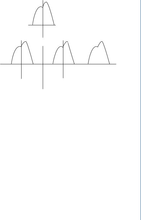
f (t)

Nonperiodic

t

0

Periodic

fT (t)

0

FIGURE 12.7: A transient pulse. Top trace is a transient; bottom trace is periodic

It is an accepted fact that a periodic function, fT (t), can be expressed as the sum of eternal exponentials of frequencies 0, ± j ω, ± j 2 ω, ±3 j ω . . . etc. Also, it is known that the Fourier Transform, Fn , amplitude of the component of frequency, jn ω, is expressed as F ( j n ω) ω 2π .

Proof of the Limiting Process: Viewing Fig. 12.7, let us examine the proof of the limiting process.

Let us begin with the general expression (12.16):

Then the exponential Fourier Series for fT (t) is given by (12.17).

n=−∞

FOURIER SERIES: TRIGONOMETRIC 139

12.9 SUMMARY

The “Forward Fourier Transform” equations are summarized in (12.22) and (12.23).

where n ω becomes a continuous variable, ω, and the function F ( j ω) is F ( j n ω).

odic function, f (t), in terms of exponential functions. The amplitude of the component of any frequency, ω, is proportional to F ( j ω). Therefore, F ( j ω), represents the frequency spectrum of f (t) and is called the Frequency Spectral of a Function. Equations (12.23) and (12.24) are referred to as the Fourier Transform pair. Equation (12.23) is the

Direct Fourier Transform of f (t), and (12.24) is the Inverse Fourier Transform.